Design effect (deff)
n/a
Exploratory Data Analysis For Epidemiology
This course was developed by Dr. Kiffer G. Card, Faculty of Health Sciences, Simon Fraser University based on Dohoo, I. R., Martin, S. W., & Stryhn, H. (2012). Methods in Epidemiologic Research. VER Inc.
📚 Reference page, available throughout the lesson
This glossary collects the key concepts, people, and ideas you will meet in this lesson. Use it as a reference while you work through the material, or as a review before assessments. Type in the search box to filter entries.
Earlier lessons systematically built up the regression toolkit for different outcome types (continuous, binary, ordered, multi-category, count, and time-to-event), but every one of those models rested on a single shared assumption: observations are independent. Real epidemiologic data almost never satisfy that assumption. Patients are nested within clinics, students within classrooms, repeated measurements within people, and households within neighbourhoods. This lesson opens the final arc of the course by taking that assumption head-on.
The four content sections build the case in stages. This section defines clustered data and catalogues the common ways it arises in public health research. A later section shows analytically why clustering breaks standard inference: standard errors collapse, Type I error rates inflate, and conclusions drift. A later section uses simulation to make the consequences tangible: you will see what happens to confidence intervals and p-values when you ignore clustering at different intra-cluster correlations. A later section previews the family of methods designed to handle clustering (mixed effects, GEE, robust/sandwich variances, and design-based survey adjustments), setting up the deeper treatment in later lessons.
In many epidemiologic studies, observations are not independent. Instead, they are grouped within higher-level units, and these groups are called clusters. Clustered (or hierarchical) data arises whenever the study design or the natural structure of the population creates groupings such that observations within the same group tend to be more similar to each other than to observations in other groups (Galbraith, Daniel, & Vissel, 2010; Killip, Mahfoud, & Pearce, 2004).
Standard statistical methods assume observations are independent. When data are clustered, this assumption is violated: observations within the same cluster share common influences (e.g., the same hospital, the same household, the same geographic region). Ignoring clustering can lead to underestimated standard errors, inflated Type I error rates, and potentially biased point estimates (Donner & Klar, 2004).
Clustering arises from many different sources. Understanding the type of clustering present in your data is the first step toward choosing an appropriate analytical strategy.
In veterinary epidemiology, animals within the same herd share management practices, nutrition, housing, and disease exposure. Similarly, patients within the same hospital share institutional protocols, staffing levels, and local disease ecology. These shared exposures create within-cluster correlation: outcomes for subjects in the same cluster are more alike than for subjects in different clusters.
People living near each other are often exposed to similar environmental factors: air pollution, water quality, neighbourhood safety, socioeconomic deprivation, and access to healthcare services. This means that health outcomes for individuals in the same geographic area are correlated. Studies that sample from defined geographic areas (e.g., census tracts, postal codes) must account for this spatial clustering.
When the same subjects are measured multiple times (e.g., before and after treatment, or at regular intervals in a cohort study), each subject forms a cluster. The repeated observations within a subject are correlated because stable individual characteristics (genetics, baseline health, behaviour) influence all measurements. The correlation structure depends on the timing and spacing of measurements.
Many real-world data structures have multiple levels. For example, students are nested within classrooms, classrooms within schools, and schools within districts. Each level contributes its own source of variation. In epidemiology, patients may be nested within physician practices, practices within health regions, and regions within provinces. Split-plot designs from experimental settings also create hierarchical structures where treatments are applied at different levels of the hierarchy.
Cross-classified structures arise when subjects belong to multiple grouping factors that do not nest within each other. For example, students may be classified by both school and neighbourhood, and students from the same neighbourhood may attend different schools, and students from the same school may live in different neighbourhoods. Split-plot designs, common in agricultural experiments, have some factors applied at the whole-plot (cluster) level and others at the subplot (individual) level.
In clustered data, the total variation in the outcome can be decomposed into between-cluster variation (differences between groups) and within-cluster variation (differences among individuals within the same group). The relative magnitude of these two sources of variation determines the strength of the clustering effect.
An important consideration is predictor clustering, which occurs when predictor variables also vary between clusters. If both the exposure and the outcome vary at the cluster level, group-level associations may differ from individual-level associations. This is the basis of the ecological fallacy: inferring individual-level relationships from aggregate (group-level) data.
1. Which is an example of clustered data?
2. What is cross-classified data?
3. Why does predictor clustering matter?
Think of a research study in your field. What natural clustering structures might exist in the data? How might ignoring this clustering affect your conclusions?
From recognising clustering to quantifying its damage. An earlier section catalogued where clustered structures come from. This section answers the natural follow-up question: so what? When observations within a cluster are even mildly correlated, the precision implied by a naive analysis, one that pretends every observation is independent, is far too optimistic. Here we develop the formal vocabulary (the intraclass correlation, the design effect, the effective sample size) that makes the size of that distortion measurable. These quantities reappear in every method we cover in a later section and in later lessons, so it is worth slowing down on the intuition.
The most important consequence of clustering is its effect on standard errors. When observations within clusters are positively correlated (as is almost always the case), treating them as independent leads to standard errors that are too small. This in turn produces test statistics that are too large, P-values that are too small, and confidence intervals that are too narrow, all of which inflate the Type I error rate.
Imagine interviewing five people from the same household about what they eat. Because they shop and cook together, the second through fifth answers mostly echo the first, so you learn far less than you would from five unrelated people. Observations within a cluster behave the same way: when they are correlated, each additional member adds only a fraction of the fresh information that a genuinely independent observation would. A naive analysis still counts every observation as fully informative, so it credits itself with more information than it actually has, which is why its standard errors come out too small.
Imagine a study of 1,000 patients in 20 hospitals (50 per hospital). If the ICC is 0.05, the design effect is 1 + (50 − 1)(0.05) = 3.45. The effective sample size is only 1,000/3.45 ≈ 290 rather than 1,000. A naive analysis treating all 1,000 observations as independent would dramatically overstate the precision of estimates.
For continuous outcomes, the ICC (intraclass correlation coefficient) measures the proportion of total variance that is attributable to between-cluster differences. It quantifies the degree of similarity among observations within the same cluster, a quantity formalised by the intraclass correlation (Killip, Mahfoud, & Pearce, 2004).
Here, σ²g is the between-cluster variance and σ² is the within-cluster variance. An ICC of 0 means no clustering effect (all variance is within clusters), while an ICC of 1 means all variance is between clusters.
The dataset phaa_clinics.csv contains 30 primary-care clinics with 18-45 patients each (~960 patients total). The continuous outcome sbp is influenced by both patient-level covariates (age, smoker, bmi) and clinic-level covariates (clinic_size, clinic_urban). The full annotated script is in r-activities/HSCI_410_Lesson_9_Introduction_to_Clustered_Data.R.
library(lme4);  library(performance);  library(sandwich);  library(lmtest)
clinics <- read.csv("phaa_clinics.csv", stringsAsFactors = FALSE)
clinics$clinic_id <- factor(clinics$clinic_id)

# 1. ICC from a one-way ANOVA
aov_fit <- aov(sbp ~ clinic_id, data = clinics)
ms     <- summary(aov_fit)[[1]][, "Mean Sq"]
n_per  <- mean(table(clinics$clinic_id))
icc_h  <- (ms[1] - ms[2]) / (ms[1] + (n_per - 1) * ms[2])
icc_h

# 2. Same ICC, conveniently, from a null mixed model
m_null <- lmer(sbp ~ 1 + (1 | clinic_id), data = clinics)
icc(m_null)

# 3. Design effect
deff <- 1 + (n_per - 1) * icc_h;  deff
nrow(clinics) / deff                          # effective sample size

# 4. Cluster-robust SEs as a quick fix for naive OLS
naive <- lm(sbp ~ age + smoker + bmi + clinic_urban, data = clinics)
coeftest(naive, vcov. = vcovCL, cluster = ~ clinic_id)
Reading the output. An ICC of about 0.08 to 0.10 means roughly 8 to 10 percent of total variation in SBP is between clinics. The design effect (here around 3.5 to 4 with average cluster size 32) tells you cluster sampling has inflated by roughly three to four times the variance you'd get under SRS. Cluster-robust SEs are the easiest fix when you can't refit the analysis as a mixed model.
Use the questions below to interpret the output you produced. Look at your console / plot before answering.
1. Report your icc_h value (from the one-way ANOVA) and the ICC from icc(m_null). Are they the same (or very close)? In one sentence, what fraction of total variance in SBP lies between clinics?
icc_h from the one-way ANOVA and icc(m_null) from the random-intercept model return nearly identical values, because both estimate the same quantity: the ratio of between-cluster variance to total variance. For this clinic dataset the ICC lands in the neighbourhood of 0.08 to 0.10, so roughly 8 to 10 percent of total variance in SBP lies between clinics and the remaining 90 percent or so is within-clinic (between individuals). This is a moderate ICC, and not unusual for a physiological measure in a multi-clinic cohort.2. Compute and report the design effect deff and the effective sample size nrow(clinics) / deff. In one sentence, explain what the deff means in practical terms (e.g., "each observation carries the information of...").
deff = 1 + (m−1)*ICC. With an average cluster size near 32 (about 960 patients across 30 clinics) and an ICC near 0.09, deff = 1 + 31×0.09 ≈ 3.8. Effective sample size = nrow(clinics) / deff ≈ 960 / 3.8 ≈ 250. Practical meaning: each clinic-clustered observation carries the information of only about 0.26 of an independent observation, so the roughly 960 rows are worth only about 250 genuinely independent ones. The design effect quantifies how much statistical power is ‘wasted’ because nearby observations within a clinic share information.3. Compare the naive OLS SEs from summary(naive)$coef[, "Std. Error"] to the cluster-robust SEs from coeftest(naive, vcov. = vcovCL, cluster = ~ clinic_id). Which predictor sees the biggest SE inflation, and why does ignoring clustering produce SEs that are too small?
The design effect (also called the variance inflation factor in the clustering context) quantifies how much the variance of an estimate is inflated due to clustering, compared to what it would be under simple random sampling (Campbell, Elbourne, & Altman, 2004).
Where m̄ is the average cluster size and ρ is the ICC. The practical meaning: if ICC = 0.05 and cluster size = 20, then deff = 1 + (20 − 1)(0.05) = 1.95, meaning the effective sample size is roughly halved.
Generate a clustered dataset (e.g., students within schools, patients within hospitals) under the null hypothesis: the treatment has no real effect. Run many simulated studies and watch how often a naive (clustering-ignoring) test wrongly declares significance. The Type I error inflation is the cost of pretending clustered data is independent.
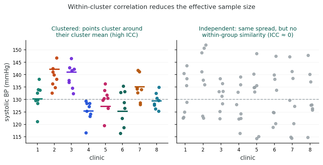
Each color = a cluster. Within-cluster similarity grows with ICC.
For continuous outcomes, the ICC directly measures the proportion of total variance due to between-cluster differences. The design effect formula deff = 1 + (m̄ − 1)ρ applies straightforwardly. The corrected standard error is obtained by multiplying the naive SE by √deff.
Example: With 20 clusters of 50 subjects each (n = 1,000), ICC = 0.05, the deff = 3.45. A naive SE of 0.50 would become 0.50 × √3.45 = 0.93, nearly double the naive estimate.
With binary or other discrete outcomes, the effects of clustering are analogous but more complex. Clustering affects the standard error estimation and can also influence point estimates. The design effect concept extends to discrete outcomes, but the ICC for binary data is defined differently and its estimation is more involved.
For binary outcomes, the variance of a proportion under clustering is inflated by a factor analogous to the deff. The practical consequence is the same: ignoring clustering leads to underestimated SEs and inflated Type I error.
| Analysis Approach | SE Estimate | 95% CI Width | P-value |
|---|---|---|---|
| Naive (ignoring clustering) | 0.50 | 1.96 | 0.001 |
| Cluster-adjusted (deff = 3.45) | 0.93 | 3.64 | 0.077 |
This table illustrates how accounting for clustering nearly doubles the standard error, widens the confidence interval, and can change a “significant” result to a non-significant one.
1. If the ICC is 0.10 and average cluster size is 21, what is the design effect?
2. What happens to Type I error rates when clustering is ignored?
3. The ICC represents:
A study reports p = 0.03 for a treatment effect, but the data come from 10 hospitals with 50 patients each. If the ICC is 0.05, calculate the design effect and discuss whether the finding might still be significant after accounting for clustering.
From formulas to felt consequences. An earlier section gave us the mathematical machinery (ICCs, design effects, effective sample sizes) that explains why clustering inflates false-positive rates. This section translates those formulas into something visceral. Simulation studies generate data with a known clustering structure and then analyse it both correctly (accounting for clusters) and incorrectly (ignoring them), so we can measure the gap directly. The takeaway you should carry forward: even small ICCs can produce alarming Type I error inflation when cluster sizes are moderate or large, and that empirical fact is what motivates the methods previewed in a later section.
Simulation studies allow us to examine the practical consequences of ignoring clustering under controlled conditions. By generating data with known clustering structures and then analysing it both correctly and incorrectly, we can quantify the bias and Type I error inflation that results from ignoring the cluster structure (Galbraith, Daniel, & Vissel, 2010; Donner & Klar, 2004).
Even moderate ICC values (e.g., 0.01–0.05) can lead to substantially inflated Type I error rates when cluster sizes are large. A study with ICC = 0.01 and 50 clusters of 50 subjects can have an actual Type I error rate of 10–15% instead of the nominal 5%. Researchers who ignore clustering risk reporting findings that appear statistically significant but are actually false positives.
Simulation studies with binary outcomes demonstrate that the consequences of ignoring clustering can be severe. Even when the ICC is small, the combination of within-cluster correlation and moderate-to-large cluster sizes can inflate the actual Type I error rate well beyond the nominal 5% level.
With ICC = 0.01 and 50 subjects per cluster, the design effect is deff = 1 + (50 − 1)(0.01) = 1.49. Although this seems modest, simulation studies show the actual Type I error rate can reach 10–15% depending on the number of clusters and the analysis method. The inflation occurs because the naive analysis assumes 50 independent observations per cluster when, in reality, the effective number is only about 34.
With ICC = 0.05 and 20 subjects per cluster, the design effect is deff = 1 + (20 − 1)(0.05) = 1.95. The effective sample size is nearly halved. Simulation studies show actual Type I error rates of 15–25% when the naive analysis is used. This means that one in four or five “significant” findings may be false positives.
With ICC = 0.10 and 30 subjects per cluster, the design effect is deff = 1 + (30 − 1)(0.10) = 3.90. The effective sample size is reduced to about one-quarter of the nominal size. Simulation studies demonstrate Type I error rates exceeding 30–40% when clustering is ignored. This level of inflation makes the naive analysis essentially unreliable.
Beyond inflating standard errors, clustering can also introduce confounding. If a cluster-level variable is associated with both the exposure and the outcome, it acts as a confounder. Failure to account for the clustering structure means this confounding is not addressed, which can lead to biased point estimates, beyond incorrect standard errors.
Suppose disease prevalence varies by region, and exposure to a risk factor also varies by region. If we analyse the data without accounting for region (the cluster), the association between exposure and disease will be confounded by regional differences. The estimated exposure effect may be biased upward or downward depending on the direction and magnitude of the confounding.
The magnitude of this bias depends on the correlation between the predictor and the cluster-level confounder. Stronger correlations produce greater bias.
1. In simulations with binary outcomes and moderate ICC, ignoring clustering:
2. How can clustering lead to confounding?
3. The inflation of Type I error due to clustering depends on:
Why might even a small ICC (e.g., 0.02) be problematic in a large cluster randomized trial with 100 participants per cluster? Calculate the design effect and discuss the implications.
From the problem to the toolkit. Earlier sections established that clustering is common, that ignoring it inflates Type I error, and that simulations make the magnitude undeniable. This section turns to the menu of solutions: fixed effects, correction factors, robust (sandwich) variance estimation, design-based survey methods, generalised estimating equations (GEE) (Liang & Zeger, 1986; Zeger & Liang, 1986), and mixed (random-effects) models (Laird & Ware, 1982; Diez Roux, 2000). Each has different strengths, different assumptions, and a different way of “paying back” the variance that clustering takes away. Treat this section as a roadmap. We will return to mixed models for continuous outcomes in a later lesson, mixed models for discrete outcomes in a later lesson, and repeated-measures designs in a later lesson.
Before choosing a method for handling clustering, you must first detect and quantify it. Common approaches include visual inspection (e.g., plotting outcomes by cluster), ICC estimation (fitting a random-intercept model to estimate the between-cluster variance), and likelihood ratio tests (comparing models with and without cluster-level random effects).
Include cluster indicators as fixed effects in the model. This effectively stratifies the analysis by cluster, adjusting for all cluster-level confounders (both measured and unmeasured). However, this approach uses many degrees of freedom (one for each cluster minus one) and does not allow estimation of cluster-level predictor effects.
Best when: There are relatively few clusters, cluster-level confounding is the primary concern, and you do not need to estimate effects of cluster-level variables.
deff-based correction: Divide test statistics by √deff or multiply standard errors by √deff. This is a simple post-hoc adjustment that requires an estimate of the ICC and the average cluster size.
Overdispersion-based correction: A similar principle using a dispersion parameter estimated from the data. The Pearson or deviance goodness-of-fit statistic divided by its degrees of freedom provides a scale factor that can be applied to the variance-covariance matrix.
Best when: A quick adjustment is needed and a more sophisticated approach is not feasible.
The robust variance estimator does not assume a specific correlation structure within clusters. It provides valid standard errors even if the within-cluster correlation is misspecified (Liang & Zeger, 1986). This makes it very attractive for practical use.
However, it requires a moderate-to-large number of clusters (rule of thumb: at least 20–30). With too few clusters, the sandwich estimator can underestimate the true variance.
Best when: You have enough clusters and want valid inference without specifying the exact correlation structure.
Survey methods account for complex sampling designs including stratification, clustering, and unequal selection probabilities (weighting). They use design-based inference rather than model-based inference, which means the validity of the analysis depends on the sampling design rather than distributional assumptions.
Available in most statistical software: Stata’s svy commands, SAS PROC SURVEY procedures, R’s survey package.
Best when: The data come from a complex survey design with known selection probabilities.
| Method | Handles Confounding | Min. Clusters | Assumptions | Software |
|---|---|---|---|---|
| Fixed Effects | All cluster-level | Few OK | None for cluster effects | All packages |
| deff Correction | No | Any | Known ICC | Manual calculation |
| Robust Variance | No | ≥20–30 | None for correlation | Stata, R, SAS |
| Survey Methods | Design-based | Varies | Known design | Stata svy, SAS PROC SURVEY, R survey |
Always check for clustering before finalising your analysis. Estimate the ICC, calculate the design effect, and choose a method appropriate to your study design and the number of clusters. When in doubt, use multiple methods and compare results. If the conclusions are consistent across approaches, you can be more confident in your findings.
1. The robust (sandwich) variance estimator:
2. When would fixed effects for clusters be most appropriate?
3. Survey methods for clustered data:
You are analyzing data from a multi-site clinical trial with 25 sites and approximately 40 patients per site. Which method(s) for handling clustering would you recommend, and why?
This lesson opened the final arc of this course by retiring the independent-observations assumption that has carried us through earlier lessons. We started by cataloguing where clustering comes from in public-health data (common environments, geography, repeated measurements, study design) and showed why it is the rule rather than the exception. Earlier sections then quantified the damage: the intraclass correlation, the design effect, and effective sample size give a precise, computable handle on how much information naive analyses pretend to have but actually don't, and simulation results made the consequences visceral.
An earlier section sketched the toolkit: fixed effects, correction factors, robust variance estimators, design-based survey methods, GEE, and mixed models. Each pays back the precision clustering takes away in a different currency, and the right tool depends on the number of clusters, whether you care about cluster-level predictors, and whether your interpretation is marginal or conditional. Later lessons take each of these approaches deeper, developing mixed models for continuous outcomes, then mixed models for discrete outcomes, and finally repeated-measures designs.
The final assessment asks you to recognise clustering on sight, compute the design effect for a sketched study, and choose a defensible analytic strategy with its trade-offs named.
Reflecting on this lesson, how has your understanding of clustered data changed? Describe a specific analytical situation where accounting for clustering would be critical and explain which method you would choose to address it.
1. Clustered data is characterized by:
2. Which is NOT a source of clustering?
3. The ecological fallacy occurs when:
4. The ICC ranges from:
5. If σ²g = 4 and σ² = 16, the ICC is:
6. A design effect of 5 means the effective sample size is approximately:
7. Ignoring clustering in analysis primarily leads to:
8. In a study with ICC = 0.05 and 40 subjects per cluster, the design effect is:
9. Cross-classified data structures differ from nested structures because:
10. Confounding by cluster occurs when:
11. The robust (sandwich) variance estimator requires:
12. Fixed effects for clusters:
13. Which statement about simulation studies on clustering is TRUE?
14. Survey methods for analyzing clustered data:
15. The deff-based correction for clustering involves:
✦ Before submitting: pass every section knowledge check (100%) and complete every reflection.