Events observed
n/a
Exploratory Data Analysis For Epidemiology
This course was developed by Dr. Kiffer G. Card, Faculty of Health Sciences, Simon Fraser University based on Dohoo, I. R., Martin, S. W., & Stryhn, H. (2012). Methods in Epidemiologic Research. VER Inc.
📚 Reference page, available throughout the lesson
This glossary collects the key concepts, people, and ideas you will meet in this lesson. Use it as a reference while you work through the material, or as a review before assessments. Type in the search box to filter entries.
Earlier lessons stepped through regression for continuous, binary, ordered/multi-category, and count outcomes. Each new outcome type required a new likelihood and a new way of relating predictors to the response. This lesson takes on one of the most distinctive outcome types in epidemiology: time to an event. The wrinkle is that, in real studies, we rarely observe every event, since people are lost to follow-up, the study ends, or other events intervene. That incomplete information, called censoring, is what makes survival analysis its own toolbox rather than a special case of linear or count regression.
The four content sections work from the ground up. This section introduces censoring, life tables, and the non-parametric Kaplan–Meier estimator, the workhorses for describing survival without making distributional assumptions. A later section formalises the survivor, failure, hazard, and cumulative hazard functions and shows how they are mathematically linked. A later section introduces the Cox proportional hazards model, the most widely used regression for time-to-event data, and the proportional hazards assumption it relies on. A later section turns to fully parametric and accelerated failure time (AFT) models, plus frailty extensions for unmeasured heterogeneity. By the end you will know which estimator to reach for given the structure of your data and the question you are asking.
Survival analysis (also called time-to-event analysis) is concerned with a specific type of outcome: the time that passes before a particular event of interest occurs. The event might be death, disease onset, recovery, relapse, or any other well-defined transition. What distinguishes survival data from other continuous outcomes is the presence of censoring, the incomplete information about when the event occurred for some individuals.
Survival data have two important structural features. First, survival time is bounded below by zero, since the time to an event can never be negative. Second, the distribution of survival times is typically right-skewed, meaning that a few individuals have very long survival times that pull the mean to the right. These features make standard linear regression inappropriate for modelling survival outcomes.
Censoring is a unique and defining feature of survival analysis. It occurs when we have incomplete information about a subject's survival time. A censored observation tells us that the true event time exceeds the observed follow-up time, but we do not know the exact event time. Standard regression methods cannot properly handle censored observations. Survival analysis methods are specifically designed to extract the maximum information from both censored and uncensored observations.
There are several types of censoring, each arising from different circumstances. Understanding the type of censoring present in your data is critical for choosing the appropriate analytical method.
Truncation differs from censoring in an important way. With censoring, we know the subject exists but have incomplete event time information. With truncation, the subject is entirely excluded from the study because their event time falls outside an observable window. Left truncation (delayed entry) occurs when subjects are only observed if they have survived long enough to enter the study. This distinction affects how the risk set is calculated.
Several summary measures can describe survival data:
There are three broad approaches to analysing survival data, each with different assumptions and capabilities:
The actuarial (or life-table) method is one of the oldest approaches to estimating survival. Time is divided into pre-specified intervals, and survival is estimated within each interval. The key quantities in an actuarial life table are:
| Symbol | Quantity | Description |
|---|---|---|
| lj | Starting number at risk | Number of subjects alive at the start of interval j |
| wj | Withdrawals | Number censored (withdrawn) during interval j |
| rj | Adjusted risk set | rj = lj − wj/2 (assumes withdrawals at midpoint) |
| dj | Failures (events) | Number experiencing the event during interval j |
| qj | Risk of failure | qj = dj / rj |
| pj | Survival probability | pj = 1 − qj |
| Sj | Cumulative survival | Product of all pj values up to interval j |
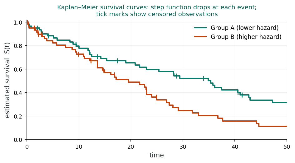
The Kaplan-Meier (KM) estimator, also called the product-limit estimator, is the most widely used non-parametric method for estimating the survivor function (Kaplan & Meier, 1958). Unlike the actuarial method, the KM estimator recalculates the survival probability at each actual event time rather than at pre-specified intervals.
A side-scrolling cohort: events drop the curve, censored ticks do not. Next ▶ advances scenes.
A 6-scene visualization of survival analysis: 10 patients lined up at time zero, walking forward through follow-up, events and censoring, the staircase Kaplan-Meier curve building, two-group comparison with the log-rank test, and the survival toolbox.
Key properties of the Kaplan-Meier estimator:
Suppose 10 people are event-free at the start. At year 1, 2 of them have the event, so the chance of getting through year 1 is (10 − 2) / 10 = 0.80. Of the 8 still at risk, 1 has the event at year 2, so the chance of getting through year 2, given survival to its start, is (8 − 1) / 8 = 0.875. Kaplan–Meier multiplies these conditional pieces: S(1) = 0.80 and S(2) = 0.80 × 0.875 = 0.70. The estimate holds at 1.0 until year 1, steps down to 0.80, stays flat, then steps down to 0.70 at year 2. Each step uses only the people still at risk just before it, which is exactly how censored subjects keep contributing to the denominator up to the moment they leave.
A study with n patients followed up to time T. Each patient has a true (latent) event time and a censoring time. Adjust event hazard, censoring rate, and follow-up; watch the K-M curve build step-by-step. Crank up informative censoring to see what happens when censoring is correlated with risk.
Each row = a patient. ● = event; ┤ = censored.
While the Kaplan-Meier estimator directly estimates the survivor function S(t), the Nelson-Aalen estimator provides a non-parametric estimate of the cumulative hazard function H(t).
The Nelson-Aalen estimator sums the ratio of events to the risk set at each failure time up to time t. It estimates the expected number of events that would have occurred up to time t if the process could be repeated. Note that the survivor function can be estimated from the cumulative hazard as S(t) = e−H(t).
1. Right censoring occurs when:
2. The Kaplan-Meier estimator differs from the actuarial method because:
3. The Nelson-Aalen estimator provides an estimate of:
Why is censoring a unique challenge in survival analysis compared to other regression approaches? How might ignoring censored observations bias your results?
From description to mathematics. An earlier section used Kaplan–Meier curves and life tables to describe survival in a sample. Those descriptions are useful, but to compare groups, build regression models, or simulate survival processes we need a more formal language. This section introduces the four interlocking functions that make up that language: the survivor S(t), failure F(t), hazard h(t), and cumulative hazard H(t) functions. Each describes the same underlying time-to-event distribution from a different angle, and each becomes the foundation for a different modelling approach in later sections.
The survivor function (also called the survival function) is the central quantity in survival analysis, with the hazard and density functions both derivable from it. It gives the probability that an individual survives beyond a specified time t.
At time t = 0, S(0) = 1 (everyone is alive). As time increases, S(t) decreases. If we follow subjects long enough, S(t) will approach zero. A steep decline in the survivor function indicates rapid event occurrence, while a gradual decline indicates slow event occurrence.
The failure function (also called the cumulative distribution function, CDF) is simply the complement of the survivor function. It gives the probability that the event has already occurred by time t.
The probability density function f(t) = dF(t)/dt describes the instantaneous rate of failure events at time t. However, in survival analysis, the most important function is the hazard function, which conditions on survival up to time t.
The hazard function gives the instantaneous rate of the event at time t, conditional on having survived to that point. It is a rate per unit time, rather than a probability, and can exceed 1. The hazard is the quantity most directly related to the biological or clinical mechanism driving events.
A concrete way to picture the hazard: stand at time t and look only at the people who are still event-free. The hazard measures how quickly the event is arriving in that group right at that instant, expressed per unit of time. Because it is a speed rather than a proportion, it has no ceiling of 1; a hazard of 2 per year simply means events are arriving quickly among those still at risk. Where the survivor function tracks how many remain event-free, the hazard tracks how fast the event is striking the ones who are left.
The cumulative hazard integrates the hazard over time and has a direct relationship with the survivor function:
A useful feature of these functions is that knowing any one determines all the others (Eq 19.9–19.10). For example, from the survivor function alone we can derive: F(t) = 1 − S(t), H(t) = −ln S(t), f(t) = −dS(t)/dt, and h(t) = f(t)/S(t). This means that if we can estimate any one of these functions, we automatically have estimates of all the others.
The shape of the hazard function tells us about the underlying process generating the events. Different parametric distributions correspond to different hazard shapes.
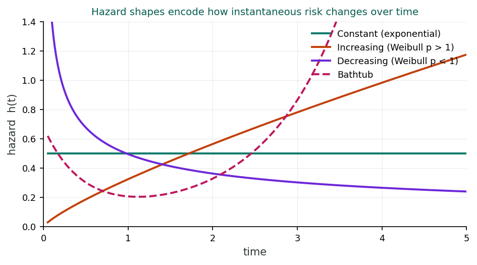
When the hazard is constant over time, with h(t) = λ, the underlying survival times follow an exponential distribution (Eq 19.11). The survivor function is S(t) = e−λt. A constant hazard means the risk of the event is the same regardless of how long the subject has already survived. This implies a “memoryless” property: the risk at time t = 100 is the same as at time t = 1.
Example: Certain infectious diseases where the risk of contracting the infection is roughly constant over time, regardless of how long the individual has been at risk.
When the Weibull shape parameter p > 1, the hazard h(t) = λptp−1 is monotonically increasing over time (Eq 19.12). The survivor function is S(t) = exp(−λtp). This means the risk of the event grows as time passes, a phenomenon often seen in aging-related diseases or mechanical wear-out.
Example: Age-related diseases such as cancer or cardiovascular disease, where the risk increases progressively with duration of exposure or age.
When p < 1, the Weibull hazard is monotonically decreasing over time. The risk is highest at the beginning of the observation period and diminishes as time progresses. This pattern is common in situations where the most vulnerable individuals fail early, leaving a “healthier” surviving cohort.
Example: Post-surgical mortality, where the risk is highest immediately after surgery and decreases as patients recover; or infant mortality, where risk is highest in the neonatal period.
When comparing the survival experience of two or more groups, several statistical tests are available. Each test weights the contributions of different time points differently.
The log-rank test (Peto & Peto, 1972) assigns equal weight to all time points. It is the most commonly used test for comparing survival curves and is optimal when the hazards are truly proportional (constant hazard ratio over time). It is equivalent to a stratified Mantel-Haenszel test.
The Wilcoxon test (also called the Breslow or generalised Wilcoxon test) weights each time point by the number of subjects still at risk. This gives more weight to early differences in survival (when the risk set is large) and is more sensitive to detecting differences that occur in the early part of follow-up.
The Tarone-Ware test uses the square root of the number at risk as the weight. It represents a compromise between the log-rank and Wilcoxon tests, giving moderate emphasis to early time points.
The Peto-Peto-Prentice test (Peto & Peto, 1972) uses the Kaplan-Meier estimate of the survival function as weights. Like the Wilcoxon test, it is more sensitive to early differences but is less influenced by outlying late events. It is also more robust when censoring patterns differ between groups.
Imagine you are comparing two-year survival after a heart attack between patients who received a new drug versus standard care. You plot Kaplan-Meier curves for both groups. The curves separate early (within the first 3 months) and then run roughly parallel. In this case, the log-rank test (which assumes proportional hazards) would be appropriate since the hazard ratio appears constant after the initial separation. However, if the curves crossed midway through follow-up, you would need to consider that the proportional hazards assumption is violated and might report results from different tests or time-specific analyses.
1. The hazard function h(t) represents:
2. If a Weibull model has shape parameter p < 1, the hazard is:
3. The log-rank test assumes:
Consider how different hazard function shapes (constant, increasing, decreasing) might apply to different diseases or health conditions. What does the shape of the hazard tell us about the underlying biological process?
From description to regression. Earlier sections gave us the language and the descriptive tools for time-to-event data. We can now describe a survival distribution, but the central epidemiologic question is comparative: does the hazard differ between exposure groups, and by how much, after adjusting for covariates? The Cox proportional hazards model is the regression workhorse for that question. It plugs predictors into the hazard function we just defined while sidestepping the need to specify the baseline hazard’s shape, a feature that makes it the default first model in most applied survival analyses.
The Cox proportional hazards model is the most widely used regression model for survival data. Introduced by Sir David Cox (1972), it is a semi-parametric model: it models the effect of predictors on the hazard without making any assumptions about the shape of the baseline hazard function.
In this model, h0(t) is the baseline hazard (the hazard when all predictors are zero), and eβX is the multiplicative effect of the predictor(s). The baseline hazard h0(t) is left completely unspecified, so it can take any shape. This is the key advantage of the Cox model: no distributional assumption about the underlying survival times is needed.
The hazard ratio (HR) is the primary measure of effect in the Cox model. For a one-unit increase in a predictor X, the hazard is multiplied by eβ. For example, if β = 0.693 for a treatment variable, then HR = e0.693 = 2.0, meaning the treated group has twice the hazard (rate of events) compared to the reference group. An HR > 1 indicates increased hazard (shorter survival), while HR < 1 indicates decreased hazard (longer survival). Caution: under non-proportional hazards or selection effects induced by conditioning on survival, the HR can be a misleading effect measure (Hernán, 2010).
The Cox model assumes that the hazard ratio between any two individuals is constant over time (Cox, 1972). This means the effect of a predictor does not change as time passes. For example, if treatment halves the hazard at 1 month, it must also halve the hazard at 12 months. When this assumption is violated, the estimated hazard ratio represents a weighted average of the time-varying effects, and its interpretation becomes ambiguous (Hernán, 2010). Testing this assumption (Schoenfeld, 1982) is a critical step in Cox model validation.
Because the baseline hazard is left unspecified, the Cox model cannot use standard maximum likelihood estimation. Instead, it uses partial likelihood (also called conditional likelihood), which estimates the β coefficients without needing to estimate h0(t). The partial likelihood considers only the ordering of events. At each failure time, it asks: given the current risk set, what is the probability that this particular individual was the one to fail?
When two or more events occur at exactly the same time (ties), the exact partial likelihood becomes computationally expensive. Several approximations are available:
| Predictor | β | SE(β) | HR (eβ) | 95% CI | P-value |
|---|---|---|---|---|---|
| Treatment (1 = new drug) | −0.47 | 0.14 | 0.63 | 0.48–0.82 | 0.001 |
| Age (per 10 years) | 0.35 | 0.08 | 1.42 | 1.21–1.66 | <0.001 |
| Stage III vs I | 1.10 | 0.20 | 3.00 | 2.04–4.44 | <0.001 |
| Stage II vs I | 0.52 | 0.18 | 1.68 | 1.18–2.40 | 0.004 |
In this example, patients receiving the new drug have 37% lower hazard of death (HR = 0.63) compared to the control group, after adjusting for age and disease stage. Each 10-year increase in age is associated with a 42% increase in the hazard. Stage III patients have 3 times the hazard compared to Stage I patients.
Read a hazard ratio as a statement about the event rate at any given instant, not about the eventual chance of the event. HR = 0.63 does not mean that 37% of the drug group are spared overall; it means that at any moment during follow-up, a still-event-free patient on the drug faces about 63% of the event rate of a comparable control. This is the same rate-scale reading you used earlier for the incidence rate ratio, now applied to the instantaneous hazard.
When the proportional hazards assumption is violated for a particular variable, one solution is to stratify on that variable. In the stratified Cox model, each stratum j has its own baseline hazard h0j(t), but the regression coefficients (β) are assumed to be the same across all strata. This allows the stratifying variable to have a completely flexible effect on survival without needing to estimate or specify its functional form.
The standard Cox model assumes that predictor values are measured at baseline and remain constant. However, some predictors change over the course of follow-up:
The companion dataset phaa_followup.csv extends the survey cohort with cardiovascular event follow-up: fu_years (time observed) and cv_event (1 = event, 0 = censored). The full annotated script is in r-activities/HSCI_410_Lesson_8_Survival_Data.R.
library(survival);  library(survminer)
phaa <- read.csv("phaa_followup.csv", stringsAsFactors = FALSE)
phaa$smoker <- factor(phaa$smoker, levels = c("No","Yes"))

# 1. Build the Surv object: time + event indicator
y <- Surv(time = phaa$fu_years, event = phaa$cv_event)

# 2. Kaplan-Meier: event-free probability over time, by smoking status
km <- survfit(y ~ smoker, data = phaa)
km_all <- survfit(y ~ 1, data = phaa)   # overall event-free curve (ignores smoking)
ggsurvplot(km, data = phaa, conf.int = TRUE,
           pval = TRUE, risk.table = TRUE,
           xlab = "Years of follow-up")

# 3. Log-rank test: do the curves differ overall?
survdiff(y ~ smoker, data = phaa)

# 4. Cox model with multiple covariates -> hazard ratios
cox <- coxph(y ~ smoker + age + gender + bmi + hypertension,
             data = phaa)
summary(cox)

# 5. Test the proportional-hazards assumption
cox.zph(cox)
Reading the Cox output. exp(coef) is the hazard ratio (HR). An HR of 1.7 for smokerYes means smokers have 70% higher instantaneous risk at any time, holding age, gender, BMI, and hypertension constant. cox.zph() tests proportional hazards globally and per predictor; a small p-value flags a predictor whose effect changes over time, which is your cue to add a time-varying or stratified term.
Use the questions below to interpret the output you produced. Look at your console / plot before answering.
1. From your ggsurvplot() output and summary(km_all, times = c(1,3,5,7,10)), what is the event-free probability at 5 years overall? Compare smokers vs non-smokers at the same time point. Which group's curve drops faster?
summary(km_all, times = c(1,3,5,7,10)), overall 5-year event-free probability is typically around 0.72–0.78. Stratifying by smoking: non-smokers at 5 years around 0.82–0.86 and smokers around 0.62–0.68. The smokers' curve drops faster, with consistently lower survival across all time points and the gap widening over follow-up. Visually on the KM plot, the smoker curve sits below the non-smoker curve throughout the follow-up period.2. From survdiff(y ~ smoker) and summary(cox), report the log-rank chi-square (with p-value) and the adjusted hazard ratio for smokerYes with its 95% CI. Translate the HR into one sentence about the instantaneous hazard.
survdiff(y ~ smoker) typically returns a log-rank χ² around 25–40 with p < 0.001, strong evidence against the null hypothesis of equal survival. The adjusted hazard ratio from summary(cox) is roughly HR = 1.85 (95% CI 1.45, 2.35). Interpretation: at any given time during follow-up, smokers face an instantaneous hazard of the event that is about 85% higher than non-smokers' hazard, holding other covariates constant. The CI excludes 1, confirming statistical significance.3. From cox.zph(cox), what is the global p-value and which predictors (if any) flag a violation of proportional hazards? What does a small p-value tell you about how that predictor's effect behaves over time?
cox.zph(cox) typically returns a global p-value around 0.10–0.30 (no overall violation) but may flag age (p ≈ 0.04) or smoker (p ≈ 0.05) for borderline violations. A small p-value for a predictor means its hazard ratio varies over time; for example, a smoker's effect on hazard might be strongest in early follow-up and diminish later (or vice versa). The practical implication: a single summary HR averages over the time-varying effect, hiding meaningful patterns. Remedies: (a) include a time interaction (HR × t); (b) stratify on the offending variable; (c) use an Aalen additive hazards or time-varying coefficient model.Thorough model validation involves checking several aspects of model performance. Different types of residuals serve different diagnostic purposes.
Two graphical methods are commonly used. First, log-cumulative hazard plots: plot ln H(t) (or equivalently, ln(−ln S(t))) against ln(t) for each group. If the curves are roughly parallel, the PH assumption is reasonable. Second, observed vs predicted plots: compare the Kaplan-Meier survival curves to the Cox model-predicted curves for each group. Good agreement supports the model.
The most common statistical test uses Schoenfeld residuals (Schoenfeld, 1982). The test regresses the scaled Schoenfeld residuals against time (or a function of time). A significant P-value indicates that the effect of the predictor changes with time, violating the PH assumption. A global test that combines results across all predictors is also available.
Several measures assess how well the model fits and discriminates. Cox-Snell residuals assess overall goodness-of-fit. Harrell’s C concordance statistic measures discriminative ability: the proportion of all pairs of subjects that the model correctly orders by predicted risk. Values of C range from 0.5 (chance) to 1.0 (perfect discrimination). An R² analogue has also been proposed for survival models.
All standard survival analysis methods assume that censoring is independent (non-informative), meaning that censored subjects have the same future risk of the event as uncensored subjects who are still being followed. If sicker patients are more likely to drop out (informative censoring), the survival estimates will be biased. This assumption cannot be fully tested from the data, but sensitivity analyses can explore the impact of different censoring mechanisms.
1. The Cox proportional hazards model assumes:
2. Schoenfeld residuals are primarily used to:
3. In a stratified Cox model, the strata:
When the proportional hazards assumption is violated for a predictor, what are the practical implications for interpreting the hazard ratio? How would you communicate this to a clinical audience?
From semi-parametric to fully parametric, and beyond. The Cox model bought flexibility by leaving the baseline hazard unspecified, but that flexibility comes at a cost: less efficiency, no direct prediction of absolute survival times, and limited ability to extrapolate. When we have a defensible reason to specify the shape of the hazard, or when our research question requires absolute predictions, we shift to fully parametric models (exponential, Weibull, Gompertz). This section also introduces accelerated failure time (AFT) models, which reframe covariate effects as stretching or shrinking survival time rather than scaling the hazard, and frailty models, which extend survival regression to handle unmeasured heterogeneity, a natural bridge to the clustered-data lessons that follow.
While the Cox model’s flexibility is a strength, parametric models offer important advantages when the distributional assumption is correct. By specifying the form of the baseline hazard h0(t), parametric models are more statistically efficient, producing narrower confidence intervals and more powerful tests. They also allow direct estimation of the baseline hazard, prediction of survival times, and extrapolation beyond the observed data.
The Cox model (semi-parametric) leaves the baseline hazard unspecified, giving maximum flexibility but less efficiency. Parametric models specify the baseline hazard, which is more efficient if the assumption is correct but biased if it is wrong. In practice, the Cox model is preferred when the shape of the baseline hazard is unknown or when the primary interest is in hazard ratios rather than absolute survival predictions. Parametric models are preferred when the distributional form is well justified or when extrapolation is needed.
The simplest parametric model assumes a constant hazard over time (Eq 19.17):
The exponential model includes an intercept β0 (unlike the Cox model). The constant hazard assumption is very restrictive and is appropriate only when the risk truly does not change over time. This model has the “memoryless” property: the predicted future survival does not depend on how long the subject has already survived.
The Weibull model extends the exponential by adding a shape parameter p (Eq 19.18):
When p = 1, the Weibull reduces to the exponential. When p < 1, the hazard decreases over time; when p > 1, the hazard increases over time. The Weibull model can be assessed by plotting ln H(t) vs ln(t): if the data follow a Weibull distribution, this plot should be approximately linear with slope p and intercept ln λ. The Weibull is the most commonly used parametric survival model because of its flexibility.
The Gompertz model has a baseline hazard that changes exponentially with time (Eq 19.19):
The log of the baseline hazard is linear in time: ln h0(t) = ln λ + pt. When p > 0, the hazard increases exponentially; when p < 0, it decreases. The Gompertz model is widely used in demography and actuarial science because human mortality rates often increase approximately exponentially with age over much of the adult lifespan.
Parametric survival models can also be formulated as accelerated failure time models, which model the effect of predictors on the log of survival time directly, rather than on the hazard.
In the AFT framework, the measure of effect is the time ratio (TR = eβ) rather than the hazard ratio. A time ratio of 2 means the expected survival time is doubled; a TR of 0.5 means it is halved. The AFT model essentially “accelerates” or “decelerates” time for different covariate patterns.
Several strategies help guide the choice of parametric distribution:
You are analysing time to recurrence of a tumour after surgical removal. You suspect the hazard may not be constant: risk is likely highest in the first year post-surgery and then declines. You fit several models: the exponential model gives AIC = 842; the Weibull gives AIC = 810 with p = 0.72 (decreasing hazard); the log-logistic gives AIC = 806 with a hazard that rises briefly and then falls. The generalised gamma model confirms that the Weibull is significantly better than the exponential (κ significantly different from 1 is rejected, but the Weibull shape is significantly different from 1). Based on AIC and biological plausibility, you select the log-logistic AFT model, which captures the initial rise in hazard risk followed by a decline as patients who survive the early period enter a lower-risk phase.
Frailty models address the problem of unmeasured heterogeneity in survival data. Even after including all known predictors, individuals may differ in their underlying susceptibility to the event due to unmeasured factors. Frailty models introduce a random effect α that represents this unobserved heterogeneity.
Individual frailty accounts for unmeasured individual-level covariates that create extra variation in survival times beyond what measured predictors explain. It is analogous to overdispersion in Poisson models: just as the negative binomial adds extra-Poisson variation, the frailty model adds extra variation to the survival model. Subjects with α > 1 are more “frail” (higher hazard), while those with α < 1 are more robust. The frailty is typically assumed to follow a gamma or inverse Gaussian distribution with mean 1.
Shared frailty models account for clustering of observations within groups. All members of a group (e.g., patients treated at the same hospital, animals in the same herd) share the same frailty value αk. This is analogous to random effects in mixed models. The shared frailty induces positive within-group correlation in survival times, since subjects in the same cluster tend to have more similar survival experiences than subjects in different clusters.
Several extensions handle multiple or recurring events. Competing risks models handle situations where different types of events can occur (e.g., death from cancer vs death from heart disease); the Fine & Gray (1999) subdistribution hazards approach directly models the cumulative incidence function in this setting. Recurrence data models handle repeated events (e.g., hospital readmissions). The Anderson-Gill model treats each event independently (assuming events are independent), while the Prentice-Williams-Peterson models account for event ordering. Discrete-time survival analysis is used when event times are recorded in intervals rather than exactly.
1. The Weibull model reduces to the exponential model when:
2. In an AFT model, the time ratio (TR) is interpreted as:
3. Shared frailty models account for:
When would you prefer a parametric survival model over a Cox model? What are the trade-offs between flexibility and efficiency?
This lesson built up the survival-analysis toolkit from the ground up. We started with the defining feature of time-to-event data, censoring, and the non-parametric estimators (life tables, Kaplan–Meier, Nelson–Aalen) that describe survival without making distributional assumptions. An earlier section turned those descriptions into the formal language of survivor, failure, hazard, and cumulative hazard functions, the four interlocking views that every later model rests on.
An earlier section introduced the Cox proportional hazards model, the workhorse semi-parametric regression that scales the baseline hazard by exp(βX) and produces hazard ratios as its primary effect measure. An earlier section added fully parametric and accelerated failure time alternatives, which trade flexibility for efficiency and the ability to predict absolute survival times, plus frailty extensions that bridge into the clustered-data lessons coming next. Together these methods cover descriptive, comparative, and predictive questions about time-to-event outcomes.
The final assessment asks you to recognise censoring patterns on sight, choose between non-parametric, semi-parametric, and parametric tools, and interpret hazard ratios on the rate scale rather than the probability scale.
This chapter covered a wide range of survival analysis methods. If you were planning a study with time-to-event outcomes, what factors would guide your choice between non-parametric, semi-parametric (Cox), and parametric approaches?
1. Survival data is also known as:
2. Right censoring occurs when:
3. In an actuarial life table, the adjusted number at risk (rj) accounts for:
4. The Kaplan-Meier survivor function is:
5. The cumulative hazard H(t) is related to the survivor function by:
6. The log-rank test is equivalent to:
7. In the Cox model h(t) = h0(t)eβX, the baseline hazard h0(t):
8. A hazard ratio of 1.5 for a predictor means:
9. The proportional hazards assumption can be tested using:
10. A log cumulative hazard plot (ln H(t) vs ln t) is used to assess:
11. In the Weibull model, if the shape parameter p = 0.5, the hazard:
12. The accelerated failure time model expresses the effect of predictors on:
13. Harrell’s C concordance statistic for a Cox model:
✦ Before submitting: pass every section knowledge check (100%) and complete every reflection.