Modelling Count and Rate Data
Exploratory Data Analysis For Epidemiology
Learning objectives for this lesson:
- Distinguish among simple counts, rates with person-time denominators, population rates, and area-based counts
- Describe the Poisson distribution and its mean=variance property
- Specify and interpret a Poisson regression model including the offset term
- Interpret incidence rate ratios (IRR) from exponentiated Poisson coefficients
- Evaluate Poisson models using Pearson, deviance, and Anscombe residuals
- Distinguish apparent from real overdispersion and apply appropriate corrections
- Compare negative binomial regression models (NB-1, NB-2) to Poisson regression
- Apply zero-inflated, hurdle, and zero-truncated models to handle excess zeros
This course was developed by Dr. Kiffer G. Card, Faculty of Health Sciences, Simon Fraser University based on Dohoo, I. R., Martin, S. W., & Stryhn, H. (2012). Methods in Epidemiologic Research. VER Inc.
Glossary: Key Terms, People & Concepts
📚 Reference page, available throughout the lesson
This glossary collects the key concepts, people, and ideas you will meet in this lesson. Use it as a reference while you work through the material, or as a review before assessments. Type in the search box to filter entries.
Introduction & The Poisson Distribution
Introduction and Overview
Earlier lessons covered regression for continuous, binary, and ordered/multi-category outcomes. This lesson takes on the next major outcome type: counts. Number of disease cases, hospital admissions, parasites, or events per unit time are all counts, and they need their own GLM family (Nelder & Wedderburn, 1972). The four content sections walk through this in order: the Poisson distribution and why it's the natural starting point (this section), Poisson regression with the offset term that lets us model rates as well as counts (a later section), residuals and the most consequential complication, overdispersion (a later section), and finally negative binomial and zero-adjusted models when standard Poisson breaks down (a later section). The offset term is the key conceptual bridge to the rate-based cohort designs you met in earlier courses and lessons.
Learning Objectives
- Distinguish simple counts, person-time rates, population rates, and area-based counts in epidemiological data.
- State the assumptions of the Poisson distribution, including the variance-equals-mean property.
- Compute Poisson probabilities and recognise the shape of the distribution at small versus large means.
- Identify when count data are likely to violate Poisson assumptions and why it matters.
Why Model Count and Rate Data?
Many outcomes in epidemiology are measured as counts, such as the number of disease cases in a region, the number of doctor visits per year, or the number of parasites on a host animal. These outcomes differ fundamentally from continuous outcomes (modelled with linear regression) and binary outcomes (modelled with logistic regression). Count data require their own family of statistical models because they are discrete, non-negative, and often right-skewed (Coxe, West, & Aiken, 2009).
Chapter 18 introduces the statistical tools for modelling count and rate data, beginning with the Poisson distribution and Poisson regression, and extending to negative binomial and zero-adjusted models for situations where the basic Poisson assumptions are violated.
Types of Count and Rate Data
Before selecting an analytical approach, it is essential to understand which type of count or rate data you are working with. There are four main types encountered in epidemiological research:
The Poisson Distribution
The Poisson distribution is the foundational probability distribution for modelling count data. It describes the probability of observing a given number of events in a fixed interval of time or space, assuming events occur independently at a constant average rate. It is the foundational distribution for the Poisson model.
From raindrops to per-minute counts to the Poisson PMF. Next ▶ advances scenes.
A 6-scene visualization of count and rate data: random events at constant rate λ, per-minute counting, the histogram filling, the Poisson PMF emerging, and the bridge to rates and rate ratios.
In this formula, Y is the count of events, μ (mu) is both the mean and the expected number of events, and e is the base of the natural logarithm (≈ 2.718). The factorial in the denominator (y!) ensures the probabilities are correctly normalised. The Poisson distribution is defined for non-negative integers: y = 0, 1, 2, 3, …
Key Property: Mean = Variance
The defining property of the Poisson distribution is that the mean equals the variance: E(Y) = Var(Y) = μ (Coxe et al., 2009). This single-parameter property means that as the expected count increases, so does the variability. This assumption is central to Poisson regression, and when it is violated (variance > mean), we have overdispersion, which requires alternative approaches covered in later sections.
The Poisson distribution is particularly useful for modelling rare events in large populations. When the probability of an event is small and the number of trials (or opportunities) is large, the Poisson distribution provides an excellent approximation. Examples include the number of rare disease cases in a large population, or the number of equipment failures over an extended operating period.
The Poisson distribution is appropriate when: (1) events are independent of one another; (2) the rate at which events occur is constant over the observation period; (3) two events cannot occur at exactly the same instant; and (4) the probability of an event in a short interval is proportional to the length of the interval. In practice, these assumptions are often approximately met in epidemiological settings.
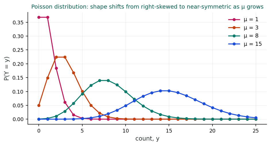
When μ is small (e.g., μ < 3), the distribution is noticeably right-skewed, with most observations clustering near zero and a long right tail. As μ increases, the distribution becomes more symmetric and begins to resemble a normal distribution. By the time μ ≥ 20, a normal approximation with mean μ and variance μ is often adequate.
1. Which type of count data uses person-time in the denominator?
2. What is the key property of the Poisson distribution?
3. The Poisson distribution is most appropriate for modelling:
Reflection
How might the type of count data (simple counts vs. rates) influence your choice of analytical approach in an epidemiological study you're familiar with?
offset(log(person_years))) is required for a chronic-disease registry where each patient contributes different person-time. Confusing the two leads to substantial bias: treating rate data as counts ignores the denominator, while treating count data as rates over-corrects for non-existent variation in exposure time.Poisson Regression Model & Interpretation
Introduction and Overview
An earlier section introduced the Poisson distribution as the probability model behind count data. This section turns the distribution into a regression. The log-linear formulation (Nelder & Wedderburn, 1972) lets us link counts to predictors on a multiplicative scale, and the offset term is the trick that converts a count model into a rate model, precisely what you need to handle person-time denominators from the rate-based cohort designs you saw in earlier courses and lessons.
Learning Objectives
- Write down a Poisson regression model with a log link and identify its linear predictor.
- Use an offset term to convert a count model into a rate model with person-time denominators.
- Interpret exponentiated Poisson coefficients as multiplicative rate ratios.
- Translate a fitted Poisson regression into incidence rates and predicted counts for new covariate values.
The Expected Count
The starting point for Poisson regression is the relationship between the expected number of events and the underlying rate. If an individual (or group) is observed for n units of person-time and the event rate is λ (lambda), the expected count is:
Here, n represents the person-time at risk (e.g., person-years of follow-up) and λ is the incidence rate. The expected count is simply the product of the time at risk and the rate at which events occur. Different subjects may contribute different amounts of person-time, which must be accounted for in the model.
The Log-Linear Model
Poisson regression uses a log link function to relate the expected count to a linear combination of predictors. Taking the natural logarithm of both sides of the expected count equation and incorporating predictors gives us the Poisson regression model:
The term ln(n) is the offset, a fixed term in the model that is included, rather than estimated, to account for the fact that different observations may have different amounts of exposure (person-time). The β coefficients describe how the log of the expected count (or rate) changes with the predictors. Fixing that coefficient at exactly 1 encodes a simple idea: a subject followed for twice as long is expected to accumulate about twice as many events, so the offset simply carries the denominator of the rate rather than being a quantity the data must estimate.
The Offset Term
The offset is one of the most important concepts in Poisson regression. It transforms the model from one that predicts counts to one that effectively predicts rates (Coxe et al., 2009).
Modelling Counts (Without Offset)
When no offset is included, the model predicts the expected count directly:
ln(E(Y)) = β0 + β1X1 + …
This is appropriate when all observations have the same amount of exposure or follow-up time. For instance, if all herds are observed for exactly one year, the count of disease cases directly reflects the rate. In practice, this situation is relatively uncommon, since most epidemiological studies have subjects with varying follow-up times.
Modelling Rates (With Offset)
When the offset ln(n) is included, the model effectively predicts the rate rather than the raw count:
ln(E(Y)) = ln(n) + β0 + β1X1 + …
This is equivalent to modelling ln(E(Y)/n) = β0 + β1X1 + …, where E(Y)/n is the expected rate. The offset accounts for the fact that subjects with longer follow-up times are expected to accumulate more events simply by virtue of being observed longer. This is the standard approach when follow-up times vary across subjects.
Interpreting Poisson Regression Coefficients
In Poisson regression, the exponentiated coefficient eβ is interpreted as an incidence rate ratio (IRR), consistent with the wider generalised linear model framework. This is analogous to the odds ratio in logistic regression but applies to rates rather than odds.
Incidence Rate Ratio (IRR)
For a one-unit increase in the predictor X1, the incidence rate is multiplied by eβ1. If β1 = 0.30, then IRR = e0.30 = 1.35, meaning the rate increases by 35% for each one-unit increase in X1. An IRR > 1 indicates an increased rate; an IRR < 1 indicates a decreased rate; and an IRR = 1 indicates no association.
Suppose we model the number of mastitis cases per herd over one year, with herd size as a predictor and cow-years at risk as the offset. The Poisson regression yields βherd size = 0.012.
Interpretation: e0.012 = 1.012, so for each additional cow in the herd, the incidence rate of mastitis increases by 1.2%. A herd with 100 more cows would have an expected rate ratio of e0.012×100 = e1.2 = 3.32 compared to the baseline, a 3.32-fold higher mastitis rate. Notice that the scaling is done on the coefficient scale first: multiply the coefficient by 100, then exponentiate. Multiplying the rate ratio itself by 100 (1.012 times 100) would be wrong, because rate ratios compound by multiplication rather than adding up.
The companion dataset phaa_followup.csv records how many GP visits each participant had during their follow-up. Because follow-up time varies, we need an offset of log(fu_years) to turn the count into a rate. The full annotated script is in r-activities/HSCI_410_Lesson_7_Count_and_Rate_Data.R.
library(MASS);  library(AER)
phaa <- read.csv("phaa_followup.csv", stringsAsFactors = FALSE)
phaa$smoker <- factor(phaa$smoker, levels = c("No","Yes"))

# 1. A peek at the count outcome
summary(phaa$gp_visits)
hist(phaa$gp_visits, breaks = 30,
     main = "GP visits during follow-up", xlab = "Visits")

# 2. Poisson regression with offset to model the RATE per person-year
fit_rate <- glm(gp_visits ~ age + smoker + hypertension
                            + offset(log(fu_years)),
                family = poisson, data = phaa)
summary(fit_rate)
exp(coef(fit_rate))                              # incidence-rate ratios
exp(confint(fit_rate))

# 3. Goodness of fit: Pearson chi^2 / df ~ 1 = good
sum(residuals(fit_rate, type = "pearson")^2) / fit_rate$df.residual

# 4. Formal overdispersion test
dispersiontest(fit_rate)

# 5. Negative binomial fall-back when Poisson is overdispersed
fit_nb <- glm.nb(gp_visits ~ age + smoker + hypertension
                              + offset(log(fu_years)), data = phaa)
AIC(fit_rate, fit_nb)
cbind(Poisson = exp(coef(fit_rate)),
      NegBin  = exp(coef(fit_nb)))
Why the offset isn't a predictor. Because its coefficient is fixed at 1, offset(log(fu_years)) shifts the intercept onto the rate scale without using a degree of freedom. The IRR for smokerYes tells you the multiplicative effect of smoking on the visit rate, holding age and hypertension constant. If dispersiontest() is significant, prefer glm.nb(); CIs widen but the point estimates are usually similar.
R Reflect on what you just ran
Use the questions below to interpret the output you produced. Look at your console / plot before answering.
1. From exp(coef(fit_rate)) and exp(confint(fit_rate)), report the IRR (and 95% CI) for smokerYes. Translate it into one sentence: how does the rate of GP visits per person-year differ between smokers and non-smokers?
exp(coef(fit_rate)) typically returns an IRR for smokerYes of about 1.40, 95% CI roughly (1.25, 1.55). Interpretation: smokers have an incidence rate of GP visits per person-year about 40% higher than non-smokers, holding other covariates constant. The CI excludes 1, so the effect is statistically significant.2. Compute sum(residuals(fit_rate, type = "pearson")^2) / fit_rate$df.residual. Is it close to 1, or much larger? Also report the p-value from dispersiontest(fit_rate). What do those two pieces of evidence say about overdispersion?
sum(residuals(fit_rate, type="pearson")^2) / fit_rate$df.residual typically returns a value around 1.4–2.0, meaningfully larger than 1, suggesting overdispersion. dispersiontest(fit_rate) gives a small p-value (typically < 0.01), confirming statistically significant overdispersion. Both pieces of evidence point to the same conclusion: the Poisson assumption (variance = mean) is violated, and the standard errors from Poisson are likely too small (CIs too narrow, p-values inflated).3. From AIC(fit_rate, fit_nb) and the side-by-side IRR comparison, which model do you prefer? Are the point estimates similar between Poisson and NegBin? What typically changes when you switch (point estimates, CIs, or both)?
AIC(fit_rate, fit_nb) typically shows AIC much lower for the negative binomial model (often hundreds of points lower), strongly favouring NegBin. The point estimates for IRRs are very similar between Poisson and NegBin, which is expected because both are estimating the conditional mean structure. What changes are the standard errors: NegBin SEs are larger (because they account for the extra variance from the over-dispersion parameter), so the CIs widen and p-values become less extreme. The lesson: overdispersion doesn't bias the point estimates much, but mis-specifying it gives over-confident inference.Poisson Regression for Relative Risk Estimation
An important application of Poisson regression is estimating relative risks (RR) directly from binary outcome data. When the outcome is rare, the Poisson model can provide estimates of the RR that are more interpretable than the odds ratios from logistic regression. This approach typically uses robust (sandwich) standard errors to account for the fact that binary data do not truly follow a Poisson distribution.
1. What is the purpose of the offset term in Poisson regression?
2. The exponentiated Poisson regression coefficient (eβ) is interpreted as:
3. Using Poisson regression to estimate relative risks from binary data is appropriate when:
Reflection
Consider a study where participants have very different follow-up times. How would using an offset term change your interpretation compared to simply modelling raw counts?
offset(log(person_years)) in a Poisson model fixes the coefficient on log(person-years) at exactly 1, effectively modelling the rate (events per person-year) rather than the raw count. Without an offset, the model would estimate a coefficient on log(person-years) that absorbs the relationship between exposure time and outcome, leaving it biased and not interpretable. With the offset, the IRRs read as multipliers on the rate (smokers have 1.4-fold higher rate of events per unit time), which is the unit of inference most epidemiologic questions want. Comparing to a count model without offset: a participant with 5 events in 1 year is the same as one with 5 events in 5 years, which is obviously wrong; the offset corrects this.Evaluating Poisson Models & Overdispersion
Introduction and Overview
An earlier section fit the Poisson model. This section turns to evaluating it. Poisson regression makes a strong assumption, that the variance equals the mean, which real count data frequently violate (Ver Hoef & Boveng, 2007). Overdispersion is the most common diagnosis you'll make on a count model, and addressing it is what a later section will be about. First, though, you need the residuals and goodness-of-fit tools to detect it.
Learning Objectives
- Compute and interpret Pearson, deviance, and Anscombe residuals from a Poisson model.
- Apply the deviance and Pearson chi-squared statistics as overall goodness-of-fit tests.
- Define overdispersion in terms of the variance-to-mean ratio and explain why it inflates Type I error.
- Choose between quasi-Poisson, scale-corrected, and negative binomial responses to overdispersion.
Residuals for Poisson Models
Just as in linear regression, residuals are the primary tool for evaluating how well a Poisson model fits the observed data. However, because the variance of a Poisson variable depends on its mean, raw residuals (observed − expected) are not directly comparable across observations. Several types of standardised residuals have been developed:
Pearson residuals standardise the raw residual by dividing by the square root of the expected value:
This accounts for the Poisson assumption that Var(Y) = μ. If the model fits well, Pearson residuals should have approximately mean 0 and variance 1. The sum of squared Pearson residuals follows an approximate χ² distribution and can be used as an overall goodness-of-fit test.
Deviance residuals are based on the contribution of each observation to the overall model deviance (the log-likelihood ratio comparing the fitted model to a saturated model). They are defined as:
di = sign(yi − μ̂i) × √[2(yi ln(yi/μ̂i) − (yi − μ̂i))]
Deviance residuals tend to be more normally distributed than Pearson residuals, especially when some expected counts are small. This makes them preferable for normal probability plots and other diagnostic displays.
Anscombe residuals use a transformation of the observed counts designed to make the residuals as close to normally distributed as possible. They apply a cube-root transformation to both the observed and expected values. Anscombe residuals are particularly useful when checking the normality assumption of residuals in Poisson models, and they complement Pearson and deviance residuals in a thorough model evaluation.
Goodness of Fit
The overall fit of a Poisson model can be assessed using the sum of squared Pearson residuals, which approximately follows a χ² distribution with (n − p) degrees of freedom, where n is the number of observations and p is the number of estimated parameters. A significant test statistic suggests the model does not fit the data adequately.
An important diagnostic is the dispersion parameter, estimated as the sum of squared Pearson residuals divided by the residual degrees of freedom:
Under the Poisson assumption (mean = variance), φ should equal 1. Values substantially greater than 1 indicate overdispersion; values less than 1 indicate underdispersion.
Why this matters in practice: when overdispersion is ignored, the Poisson standard errors come out too small, so confidence intervals are too narrow and p-values too extreme. The practical risk is calling an association statistically significant when the data do not really support it.
Understanding Overdispersion
Overdispersion, the situation where the observed variance exceeds the Poisson-assumed variance, is one of the most common problems in count data modelling (Ver Hoef & Boveng, 2007). It is critical to distinguish between two types:
Warning: Interpreting Overdispersion
Before concluding that overdispersion is “real,” always investigate whether the model is correctly specified. Adding missing predictors, removing outliers, or modelling non-linear effects may resolve apparent overdispersion without needing to change the distributional assumptions. Applying overdispersion corrections to a misspecified model can mask important features of the data.
Apparent Overdispersion
Apparent overdispersion arises from problems with the model rather than the data-generating process itself. Common causes include:
- Outliers: A few extreme observations can inflate the dispersion statistic dramatically.
- Missing important predictors: If key covariates are omitted from the model, the unexplained variation appears as overdispersion.
- Wrong model form: Using a linear predictor when the true relationship is non-linear.
- Non-linear effects: Failing to include quadratic or other polynomial terms for predictors with curvilinear relationships.
Apparent overdispersion can be resolved by correcting the model specification: removing outliers, adding missing predictors, or using the correct functional form.
Real Overdispersion
Real overdispersion reflects genuine extra-Poisson variation in the data that cannot be explained by observable covariates. This often arises from:
- Unobserved heterogeneity: Subject-level variation in the underlying rate that is not captured by measured predictors.
- Clustering: Events within groups (e.g., animals within herds) are correlated, violating the independence assumption.
- Biological variability: Inherent variation in susceptibility or exposure that exceeds what the Poisson model allows.
Real overdispersion requires statistical corrections such as scaling standard errors, using negative binomial regression, or employing random effects models.
Approaches to Handling Overdispersion
| Approach | How It Works | When to Use |
|---|---|---|
| Scale SEs by √φ | Multiplies standard errors by the square root of the estimated dispersion parameter; coefficients unchanged | Mild to moderate overdispersion; quick fix when coefficient estimates are trusted |
| Negative binomial regression | Adds an extra parameter (α) to model the excess variance explicitly | Moderate to severe overdispersion; when a more principled model is desired |
| Random effects / GLMM | Includes subject- or group-level random intercepts to capture unobserved heterogeneity | Clustered data (e.g., animals within herds); hierarchical study designs |
| GEE (robust SEs) | Uses generalised estimating equations with an empirical (sandwich) variance estimator | Clustered data when marginal (population-averaged) estimates are of primary interest |
1. In a Poisson model, overdispersion is indicated when:
2. Which of the following is NOT a cause of apparent overdispersion?
3. One approach to handling real overdispersion is:
Reflection
Why is it important to distinguish between apparent and real overdispersion before choosing a correction strategy? What could go wrong if you apply the wrong fix?
Negative Binomial & Zero-Adjusted Models
Introduction and Overview
An earlier section named overdispersion as the most common problem with Poisson regression. This section closes the lesson with the standard fixes: the negative binomial distribution (which adds a free dispersion parameter; Ver Hoef & Boveng, 2007), and zero-adjusted models for the special case where there are far more zeros than Poisson or negative binomial alone can accommodate (Lambert, 1992).
Learning Objectives
- Derive the negative binomial as a Gamma-mixed Poisson and contrast NB-1 and NB-2 parameterisations.
- Fit a negative binomial regression and compare it to a Poisson fit using a likelihood-ratio test on the dispersion parameter.
- Identify zero-inflation versus zero-truncation and choose the appropriate zero-adjusted model.
- Interpret a hurdle or zero-inflated model in terms of separate processes for the zero and the count components.
The Negative Binomial Distribution
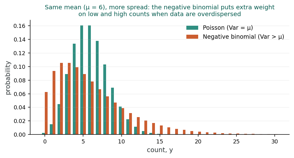
The negative binomial (NB) distribution extends the Poisson by adding an extra parameter α that captures the additional variation not accounted for by the Poisson assumption. Conceptually, the NB distribution arises when the Poisson rate itself varies randomly across individuals, so each subject has their own λ, drawn from a Gamma distribution. Averaging over those rates produces the negative binomial distribution.
The NB distribution allows the variance to exceed the mean, making it the natural first choice when overdispersion is present (Ver Hoef & Boveng, 2007). Two common parameterisations define how the variance relates to the mean:
NB-1: Linear Variance
In the NB-1 parameterisation, the variance increases linearly with the mean. The overdispersion is proportional to the mean: doubling the expected count doubles the excess variance. The ratio Var(Y)/μ = (1 + α) is constant across all observations, making NB-1 similar to a quasi-Poisson model with a fixed dispersion parameter.
NB-1 is sometimes preferred when overdispersion is relatively constant across the range of predicted values. However, it is less commonly used in practice than NB-2.
NB-2: Quadratic Variance
In the NB-2 parameterisation (the most commonly used form), the variance increases quadratically with the mean. Observations with higher expected counts have proportionally more overdispersion. This is often more realistic in biological settings where variability tends to grow faster than the average.
The NB-2 model is the default in most statistical software (e.g., Stata’s nbreg, R’s glm.nb()). When α = 0, the NB-2 model reduces to the Poisson model, making the Poisson a special (nested) case of NB-2.
Negative Binomial Regression
The NB regression model uses the same log-linear form as Poisson regression; the only difference is in the assumed distribution of the outcome:
Coefficients are interpreted identically to Poisson regression: eβ gives the incidence rate ratio. The key advantage is that the NB model produces correct standard errors even when overdispersion is present, because the extra variation is explicitly modelled through α.
Testing Poisson vs. Negative Binomial
Since the Poisson model is nested within the NB model (when α = 0), a likelihood ratio test (LRT) can be used to determine whether the NB model provides a significantly better fit. A significant LRT indicates that overdispersion is present and the NB model is preferred. Note that this is a boundary test (testing α = 0 vs. α > 0), so the p-value from the standard χ² reference distribution is conservative.
Zero-Adjusted Models
Standard count models (Poisson and NB) may not adequately handle datasets with an unusual number of zeros (Lambert, 1992). Three families of models have been developed to address different zero-related problems:
Choosing Among Zero-Adjusted Models
The choice depends on the data-generating process:
- If some zeros are “structural” (from a fundamentally different process) and others arise from the count process, use a zero-inflated model.
- If the zero/non-zero distinction is a separate decision from the magnitude of the count, use a hurdle model.
- If zeros are impossible by design, use a zero-truncated model.
| Model | Source of Zeros | Key Feature | Test / Comparison |
|---|---|---|---|
| Zero-Inflated | Both components (structural + count) | Mixture of logistic + count model | Vuong test vs. standard model |
| Hurdle | Binary component only | Two-part: binary then truncated count | LRT or AIC/BIC comparison |
| Zero-Truncated | Zeros cannot occur | Conditional on Y > 0 | Applied when sampling excludes zeros |
1. The NB-2 model differs from the Poisson model by:
2. Zero-inflated models are appropriate when:
3. The key difference between a hurdle model and a zero-inflated model is:
Reflection
When might you choose a hurdle model over a zero-inflated model in practice? Think of an epidemiological example where the distinction matters.
Lesson 7: Comprehensive Assessment
Bringing It All Together
This lesson assembled the count-and-rate toolkit. We started with the Poisson distribution and used its log-link form to build a regression, then introduced the offset term, the small piece of arithmetic that converts a count model into a rate model and unifies the cohort and incidence-density designs you have already met. From there we moved to evaluation: Pearson, deviance, and Anscombe residuals; goodness-of-fit tests; and the variance-to-mean comparison that makes overdispersion visible.
An earlier section introduced the standard responses to overdispersion. Negative binomial regression adds a dispersion parameter and is the everyday workhorse when Poisson assumptions break. Zero-adjusted models (hurdle and zero-inflated) handle outcomes where the data-generating process has separate components for whether an event occurs at all and how often it occurs given that it can. Together these models cover the bulk of count-data analyses you are likely to read or run.
The final assessment asks you to recognise count and rate situations on sight, reach for the right model, and report rate ratios with appropriate uncertainty. Use the diagnostic flowchart from an earlier section as your default answer to “which model?”.
Key Takeaways from this lesson
- Counts and rates are a distinct outcome family with their own GLM: the Poisson, with a log link.
- The offset term turns a count model into a rate model by absorbing person-time or population denominators.
- Exponentiated coefficients in Poisson and negative binomial regression are rate ratios, interpreted multiplicatively.
- Overdispersion (variance exceeding the mean) is the most common Poisson failure mode and inflates Type I error if ignored.
- Negative binomial regression is the default fix; use it whenever the dispersion test rejects Poisson.
- Zero-inflated and hurdle models handle outcomes with a separate “at-risk” process generating excess zeros.
Reflection
Reflecting on the full range of count and rate models covered in this lesson, how would you decide which model to use for a new dataset? What diagnostic steps would you follow?
Final Knowledge Assessment
1. Which type of count data involves dividing event counts by accumulated person-time?
2. The Poisson distribution assumes:
3. In Poisson regression, the offset term represents:
4. The exponentiated coefficient from a Poisson regression (eβ) is interpreted as:
5. Pearson residuals for Poisson regression are calculated as:
6. A dispersion parameter of 3.5 in a Poisson model suggests:
7. Which is a cause of APPARENT (not real) overdispersion?
8. Scaling standard errors by √φ addresses overdispersion by:
9. The NB-2 model specifies the variance function as:
10. To test whether negative binomial regression provides a better fit than Poisson, you use:
11. A zero-inflated Poisson model combines:
12. The Vuong test is used to:
13. In a hurdle model, zero counts are generated by:
14. Zero-truncated models are appropriate when:
15. Poisson regression can be used to estimate relative risks directly from binary outcome data because:
✦ Before submitting: pass every section knowledge check (100%) and complete every reflection.