Modelling Ordinal & Multinomial Data
Exploratory Data Analysis For Epidemiology
Learning objectives for this lesson:
- Select an appropriate model (multinomial, proportional-odds, adjacent-category, or continuation-ratio) based on study objectives and data
- Fit all of the models listed above
- Evaluate the assumptions on which each model is based
- Interpret OR estimates from each model
- Compute predicted probabilities from each model
This course was developed by Dr. Kiffer G. Card, Faculty of Health Sciences, Simon Fraser University based on Dohoo, I. R., Martin, S. W., & Stryhn, H. (2012). Methods in Epidemiologic Research. VER Inc.
Glossary: Key Terms, People & Concepts
📚 Reference page, available throughout the lesson
This glossary collects the key concepts, people, and ideas you will meet in this lesson. Use it as a reference while you work through the material, or as a review before assessments. Type in the search box to filter entries.
MASS::polr fits proportional-odds models; VGAM::vglm handles a broader family including partial-PO and continuation-ratio.
Introduction & Overview of Models
Introduction and Overview
An earlier lesson covered logistic regression for binary outcomes. This lesson extends the framework to outcomes with more than two categories, whether nominal (no natural order) or ordinal (ordered). The four content sections walk through the major models in order: an overview of the four-model toolkit (this section), the multinomial logistic model for nominal outcomes (a later section), the proportional-odds model for ordinal outcomes including how to test the proportional-odds assumption (a later section), and finally adjacent-category and continuation-ratio models as alternatives when proportional-odds doesn't hold (a later section). For an epidemiology-focused overview that maps all four models onto the same dataset, see Ananth & Kleinbaum (1997); the open-access encyclopedia entries on ordinal regression and multinomial logistic regression summarise the same toolkit at an undergraduate level.
Learning Objectives
- Distinguish nominal from ordinal outcomes and explain why each calls for a different modelling strategy.
- Map the four logits used by multinomial, proportional-odds, adjacent-category, and continuation-ratio models.
- Use the Apgar-score example to anticipate how each model will partition the same outcome.
- Choose an initial model based on the structure and ordering of the outcome categories.
When Outcomes Have More Than Two Categories
In many epidemiological studies the outcome variable has more than two categories. These outcomes fall into two broad types: nominal data, where the categories have no natural ordering (e.g., type of disease, preferred clinic), and ordinal data, where the categories are ordered (e.g., pain severity: none, mild, moderate, severe).
The choice of model depends on whether the outcome is nominal or ordinal. Nominal data require multinomial logistic regression or log-linear models. Ordinal data can be analysed with the same multinomial model (ignoring the ordering), but more efficient approaches exploit the ordering: proportional-odds, adjacent-category, and continuation-ratio models (McCullagh, 1980; Ananth & Kleinbaum, 1997).
The Apgar Score Example
Throughout Chapter 17, the authors use Apgar scores as a running example. Apgar scores (measured at birth) are recoded into four ordinal categories. The research question is whether the number of prenatal visits is associated with Apgar score category.
| Apgar Category | Code | Prenatal Visits < 6 | Prenatal Visits ≥ 6 | Total |
|---|---|---|---|---|
| 1–6 (Low) | 0 | 47 | 25 | 72 |
| 7 | 1 | 48 | 42 | 90 |
| 8 | 2 | 59 | 72 | 131 |
| 9–10 (High) | 3 | 134 | 227 | 361 |
| Total | 288 | 366 | 654 |
Overview of the Four Models
Each of the four models for multi-category outcomes uses a different formulation of the logit (log-odds). Understanding the logit structure is the key to understanding each model.
Compares each outcome category to a baseline category. For J categories, the model estimates J−1 sets of coefficients. Each set describes how predictors relate to the log-odds of being in category j versus the baseline.
No assumptions about ordering are made, so this model is appropriate for both nominal and ordinal outcomes (though it is less efficient for ordinal data).
Based on cumulative probabilities. The logit compares the probability of being at or above category j versus below it. A single coefficient per predictor applies at every cutpoint, the proportional-odds assumption.
This is the most common ordinal logistic model and is more parsimonious than the multinomial model (McCullagh, 1980).
Compares each category to the adjacent (next lower) category. This model is a constrained version of the multinomial model where the coefficient for categories n levels apart equals n times the coefficient for adjacent categories.
Like the proportional-odds model, it estimates a single β1 per predictor.
Compares each category to all lower categories combined. This model is especially appropriate when the outcome represents sequential stages that must be “passed through” to reach higher levels (e.g., number of attempts to achieve certification).
Can be fit as a series of separate binary logistic regressions with appropriately recoded outcome variables.
1. Nominal outcome data differ from ordinal outcome data in that:
2. How many sets of coefficients does a multinomial logistic model estimate for J outcome categories?
3. Which model assumes the effect of a predictor is the same across all cutpoints?
✎ Reflection
Think of an ordinal outcome variable from your own field of study. What are the categories, and which of the four models introduced here do you think would be most appropriate? Why?
Multinomial Logistic Regression
Introduction and Overview
An earlier section mapped the four-model landscape. This section walks into the first one in detail: the multinomial logistic model. This is the most general option: it works on any categorical outcome, ordered or not, but you pay for that generality with a coefficient for every comparison and many more parameters to interpret.
Learning Objectives
- Set up a multinomial logistic model as J−1 simultaneous binary logits against a chosen baseline.
- Interpret exponentiated coefficients as relative risk ratios for non-baseline versus baseline categories.
- Compute predicted probabilities for every outcome category from the joint set of linear predictors.
- Recognise the independence-of-irrelevant-alternatives (IIA) assumption and its implications.
The Multinomial Logistic Model
The multinomial logistic model simultaneously fits J−1 separate logistic models, each comparing one category to a chosen baseline. All parameters are estimated jointly, so the model accounts for the correlation among the comparisons.
Predicted Probabilities
The predicted probability for each outcome category is computed from the set of linear predictors. Let Xβ(j) denote the linear predictor for category j.
These probabilities always sum to 1 across all categories. Each predicted probability depends on all sets of coefficients, rather than only the coefficients for that category.
These formulas write category 0 as the baseline for illustration. In the Apgar results below, the high category (9–10, coded 3) is used as the reference instead. Which category you call the baseline is a labelling choice: it re-expresses the coefficients but leaves the fitted probabilities and the overall fit unchanged.
Interpreting Odds Ratios
Exponentiated coefficients from a multinomial model are technically ratios of relative risks (RRR), not true odds ratios. Each exp(β(j)) gives the ratio of the probability of being in category j relative to the baseline, for a one-unit change in the predictor.
Read intuitively, a relative-risk ratio of 0.24 means that for mothers with six or more prenatal visits, the risk of the low category measured against the high baseline category is about a quarter of what it is for mothers with fewer visits. The name relative-risk ratio, rather than odds ratio, is a reminder that the comparison is built from probabilities taken against the baseline, not from odds.
Because the multinomial model estimates separate coefficients for each comparison, the effects can differ across categories. For ordinal outcomes, you would typically expect a gradient, with more pronounced effects for the categories furthest from the baseline.
Predicted Probabilities
Predicted probabilities from a multinomial model vary by the values of all predictors. To communicate results, it is often useful to compute predicted probabilities at specific covariate patterns (e.g., prenatal visits < 6 vs ≥ 6) and present them in a table or graph.
Testing significance can be done with Wald tests (for individual coefficients) or likelihood-ratio tests (for overall effects). Because the multinomial model has J−1 coefficients per predictor, an overall LRT that tests all J−1 simultaneously is generally preferred over examining individual coefficients.
Independence of Irrelevant Alternatives (IIA)
The multinomial logistic model assumes IIA: the odds of choosing one category over another are independent of what other categories are available. If this assumption is violated, adding or removing a category would change the odds between the remaining categories.
Two tests are available: the Hausman-McFadden test and the Small-Hsiao test. However, these tests often give conflicting results, and IIA violations are primarily a concern for nominal data where alternatives are genuinely substitutable (e.g., choosing a mode of transport). For ordinal data, the independence of irrelevant alternatives is rarely a practical concern.
In the Apgar score example, the multinomial model (with category 3 [9–10] as baseline) produced the following key results for prenatal visits (≥6 vs <6):
- Category 0 vs 3: OR = 0.24, so those with ≥6 visits have 76% lower relative risk of a low Apgar score
- Category 1 vs 3: OR = 0.65, a 35% lower relative risk of Apgar = 7
- Category 2 vs 3: OR = 0.72, a 28% lower relative risk of Apgar = 8
The gradient (0.24 → 0.65 → 0.72) shows the strongest effect for the lowest Apgar category, as expected for an ordinal outcome.
Note on IIA Tests
The Hausman-McFadden and Small-Hsiao tests for IIA often give conflicting results and are not always reliable. In practice, IIA is mainly a concern for nominal (unordered) outcomes with genuinely substitutable alternatives. For ordinal outcomes, it is rarely problematic. Regression diagnostics can be performed by fitting ordinary logistic models for pairs of categories and using standard diagnostic techniques.
Alternative-Specific Data
In some situations, predictors may vary across alternatives rather than (or in addition to) varying across observations. For example, in a study of clinic choice, the distance to each clinic varies by alternative. Special formulations of the multinomial model (conditional logit or mixed logit) accommodate such alternative-specific data.
1. In multinomial logistic regression, the exponentiated coefficients represent:
2. The IIA assumption states that:
3. How are predicted probabilities computed from a multinomial model?
✎ Reflection
Consider the Apgar score example. Why do you think the OR for the lowest Apgar category (0.24) is more extreme than for the middle categories? What does this gradient tell us about prenatal care and birth outcomes?
Proportional-Odds Model
Introduction and Overview
An earlier section used multinomial logistic regression to fit a model that ignores any ordering in the outcome categories. This section takes the more parsimonious route: when the categories are ordered, the proportional-odds model uses far fewer parameters by assuming the effect of each predictor is the same across all category cut-points. The trade-off is that you have to verify the proportional-odds assumption holds.
Learning Objectives
- Express the proportional-odds (cumulative logit) model in terms of an underlying latent continuous variable and cutpoints.
- Interpret a single odds ratio as the effect of a predictor across every dichotomisation of the ordinal outcome.
- Test the proportional-odds assumption using the score (Brant) test or by comparing nested models.
- Diagnose what to do when proportional-odds clearly fails for a given predictor.
The Most Common Ordinal Model
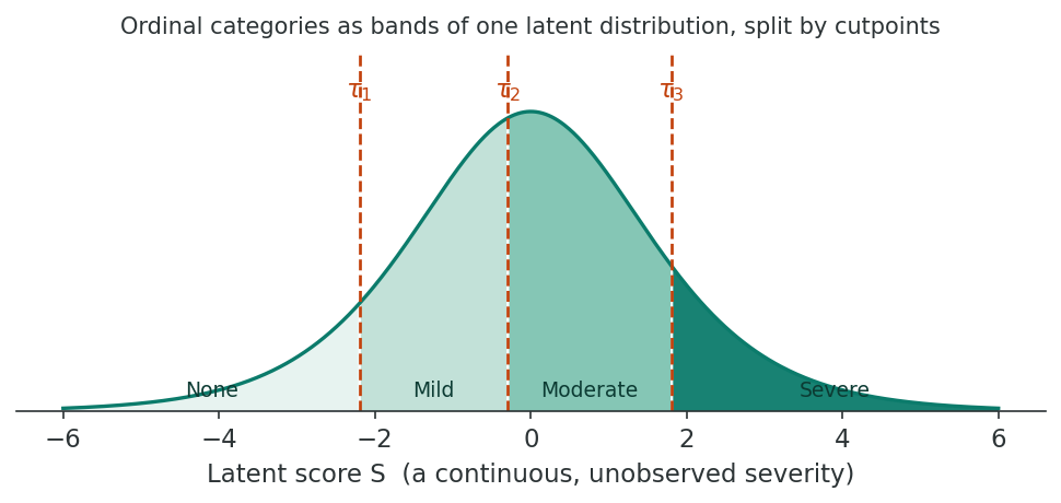
The proportional-odds model (also called the cumulative logit model or ordinal logistic regression) is the most widely used model for ordinal outcomes. It was formalised by McCullagh (1980) and is based on the idea of an underlying continuous latent variable that is divided into the observed ordinal categories by a series of cutpoints, the structure of the ordered logit model.
The latent variable Si is divided by cutpoints (τ1, τ2, …, τJ−1) into J observed categories. If Si falls between τj−1 and τj, the observation is classified into category j.
The Proportional-Odds Logit
The model takes the form of a cumulative logit: logit(p(Y ≥ j)) = β0j + βX. The key feature is that the intercept varies across cutpoints (giving parallel lines on a logit scale) but the slope coefficients are the same for every cutpoint. This means a single OR summarises the effect of each predictor across all levels of the outcome (McCullagh, 1980).
Proportional odds in plain words. The predictor multiplies the odds by the same amount wherever you split the ordered outcome. If six or more prenatal visits multiply the odds of scoring above the lowest Apgar category by 1.59, they multiply the odds of reaching the top category by that same 1.59. You get a single odds ratio, and it applies at every cutpoint. That economy is the reason to reach for the model, and the proportional-odds assumption is the one thing you have to check before trusting it.
In the Apgar score example, the proportional-odds model yields an OR of 1.59 for prenatal visits (≥6 vs <6). This means that individuals with 6 or more prenatal visits have 1.59 times the odds of being at or above any given Apgar category, compared to those with fewer visits. This single OR applies at every cutpoint (0 vs 1+, 0–1 vs 2+, and 0–2 vs 3).
The course dataset phaa_survey_clean.csv has both an unordered multi-category variable (region, 5 Lower-Mainland regions) and an ordered one (education, 5 levels). The full annotated script is in r-activities/HSCI_410_Lesson_6_Ordinal_and_Multinomial_Models.R.
library(nnet);  library(MASS);  library(brant)
phaa <- read.csv("phaa_survey_clean.csv", stringsAsFactors = FALSE)
phaa$region    <- relevel(factor(phaa$region), ref = "Vancouver")
phaa$education <- factor(phaa$education,
  levels = c("Less than high school", "High school", "Some college",
             "Bachelor's", "Graduate degree"),
  ordered = TRUE)

# 1. MULTINOMIAL: nominal outcome (region)
mn <- multinom(region ~ age + gender + smoker, data = phaa, trace = FALSE)
exp(coef(mn))                                           # relative-risk ratios
z <- summary(mn)$coefficients / summary(mn)$standard.errors
round((1 - pnorm(abs(z))) * 2, 3)                          # p-values

# 2. PROPORTIONAL-ODDS: ordered outcome (education)
po <- polr(education ~ age + gender + smoker, data = phaa, Hess = TRUE)
exp(cbind(OR = coef(po), confint(po)))                  # OR + 95% CI

# 3. Brant test: is the proportional-odds assumption defensible?
brant(po)

# 4. Multinomial fit of the SAME ordered outcome, the fall-back to compare
mn_edu <- multinom(education ~ age + gender + smoker, data = phaa, trace = FALSE)
AIC(po, mn_edu)                                        # lower AIC = better-fitting model
Reading the multinomial output. The relative-risk ratios from multinom() compare each region to the reference (Vancouver). For polr(), a single OR per predictor applies between every adjacent pair of education levels; that is the proportional-odds assumption that brant() tests. If the Brant overall p-value is < .05, compare AIC(po, mn_edu) and prefer the multinomial fit when its AIC is clearly lower (or fit a partial-PO model in the stretch).
R Reflect on what you just ran
Use the questions below to interpret the output you produced. Look at your console / plot before answering.
1. From exp(coef(mn)) and the matching p-value matrix, pick one non-reference region (anything but Vancouver) and one predictor (e.g., smokerYes). Report the relative-risk ratio, and state in one sentence what it says about the relative likelihood of living in that region versus Vancouver.
2. From exp(cbind(OR = coef(po), confint(po))), report the OR for age and its 95% CI. Under the proportional-odds assumption, translate this OR into a sentence about being at-or-above any given education level.
3. Look at the brant(po) output. What is the overall p-value, and do any individual predictors flag a violation (p < .05)? Based on this, would you keep po or fall back to mn_edu (compare AICs)?
brant() typically returns an overall p-value around 0.01–0.05; if the global is significant, some individual predictors will also show p < .05, indicating violation of the proportional-odds assumption. If violations are flagged: (a) compare AIC of po vs. mn_edu (the multinomial alternative); (b) if mn_edu has substantially lower AIC, prefer the multinomial; (c) alternatively, fit a partial proportional odds model that relaxes the assumption only for the violating predictors. The cleanest practical move when the assumption is violated and the categories are ordered is the partial proportional-odds model; its category-specific slopes let the flagged predictors act differently at each cutpoint while the outcome's ordering is preserved.Testing the Proportional-Odds Assumption
The proportional-odds assumption is that the effect of each predictor is the same at every cutpoint. If violated, the model may give misleading results. Several tests are available:
Three main approaches exist:
- Approximate LRT: Compare the log-likelihoods of the proportional-odds model and the multinomial model. A significant difference suggests the proportional-odds assumption is violated.
- Wolfe-Gould approximate LRT: Based on J−1 separate binary logistic models at each cutpoint. Sum the log-likelihoods and compare to the proportional-odds model.
- Brant (Wald) test: Provides both an overall test and individual tests for each predictor, showing which specific variables violate the assumption (Brant, 1990).
If the proportional-odds assumption is violated, a generalised ordinal logistic regression model allows separate coefficients at each cutpoint. This model is equivalent to fitting J−1 separate binary logistic regressions simultaneously. It is more flexible but less parsimonious than the proportional-odds model (Williams, 2006).
A compromise approach is the partial proportional-odds model, which relaxes the proportional-odds assumption for selected predictors only (those that fail the Brant test) while maintaining it for the rest (Peterson & Harrell, 1990; Williams, 2006). This provides a good balance between flexibility and parsimony. Other alternatives include the stereotype logistic model and the heterogeneous choice logistic model.
⚠ The Proportional-Odds Assumption in Practice
The proportional-odds assumption is often violated in practice, especially with many predictors or when the outcome categories represent very different phenomena. Always test this assumption before reporting results from a proportional-odds model (Brant, 1990). If violated, consider a partial proportional-odds model or generalised ordinal logistic regression (Peterson & Harrell, 1990; Williams, 2006).
Brant Test Results Example
The Brant test provides both an overall test and predictor-specific tests. Here is an example of how results might be presented:
| Predictor | χ² | df | P-value | Assumption Holds? |
|---|---|---|---|---|
| Prenatal visits | 2.14 | 2 | 0.343 | Yes |
| Maternal age | 8.92 | 2 | 0.012 | No |
| Parity | 1.03 | 2 | 0.598 | Yes |
| Overall | 12.45 | 6 | 0.053 | Borderline |
In this example, only maternal age violates the assumption. A partial proportional-odds model that allows maternal age to have different effects at each cutpoint (while constraining prenatal visits and parity) would be appropriate.
Regression Diagnostics
Regression diagnostics for the proportional-odds model can be conducted by fitting binary logistic models at each cutpoint and applying the diagnostic techniques from Chapter 16 (residual analysis, influence measures, goodness-of-fit tests).
1. The proportional-odds model assumes:
2. If the proportional-odds assumption is violated for some but not all predictors, which model can be used?
3. The latent variable in a proportional-odds model represents:
✎ Reflection
Why do you think the proportional-odds assumption is so often violated in practice? Can you think of a scenario in your own research where you would expect the effect of a predictor to differ across cutpoints?
Adjacent-Category & Continuation-Ratio Models
Introduction and Overview
The proportional-odds model is the workhorse for ordered outcomes, but its proportional-odds assumption is genuinely restrictive and frequently fails in real data. This section closes the lesson with two alternatives that relax that assumption in different ways: the adjacent-category model and the continuation-ratio model. Each is appropriate for a different kind of ordering and a different research question.
Learning Objectives
- Specify the adjacent-category model and test its constraint against an unconstrained multinomial fit.
- Specify the continuation-ratio model and recognise the sequential-stage outcomes it suits.
- Fit a continuation-ratio model as a series of binary logistic regressions on recoded data.
- Choose between proportional-odds, adjacent-category, and continuation-ratio models based on the question and the data.
Adjacent-Category Model
The adjacent-category model compares the probability of being in category j versus category j−1 (the next lower category). It is a constrained version of the multinomial logistic model: the constraint is that the coefficient for categories n levels apart equals n times the coefficient for adjacent categories.
Like the proportional-odds model, the adjacent-category model estimates a single β1 per predictor, making it more parsimonious than the unconstrained multinomial model. The validity of this constraint can be tested by comparing the adjacent-category model to the unconstrained multinomial model using a likelihood-ratio test (LRT) (Ananth & Kleinbaum, 1997).
For the Apgar score data, the LRT comparing the adjacent-category model to the unconstrained multinomial model yielded χ² = 6.76, df = 5, P = 0.239. Since this is not significant, the adjacent-category model is a valid simplification of the multinomial model for these data.
Continuation-Ratio Model
The continuation-ratio model compares the probability of being in category j versus all lower categories combined. It is particularly useful when the outcome represents sequential stages that must be “passed through” to reach higher levels (Ananth & Kleinbaum, 1997).
When Is the Continuation-Ratio Model Appropriate?
The continuation-ratio model is ideal for outcomes where each level must be reached before the next can be attained. Examples include: number of attempts to pass an exam, stages of disease progression where remission must occur before relapse, or sequential rounds of a selection process. It is NOT appropriate when movements between categories are not sequential (e.g., Apgar scores, where a baby does not “pass through” each score level).
Fitting the Continuation-Ratio Model
The continuation-ratio model can be fit as a series of separate binary logistic regressions with a recoded outcome variable. For each comparison:
- Y = 1 for the level of interest
- Y = 0 for all lower levels
- Observations at higher levels are excluded (treated as missing)
Consider an example with 4 categories representing the number of attempts to gain admission to medical school (1, 2, 3, 4+):
| Original Category | Y1 (1 vs 0) | Y2 (2 vs 0–1) | Y3 (3 vs 0–2) |
|---|---|---|---|
| 0 (1 attempt) | 0 | 0 | 0 |
| 1 (2 attempts) | 1 | 0 | 0 |
| 2 (3 attempts) | – | 1 | 0 |
| 3 (4+ attempts) | – | – | 1 |
You can fit either a constrained version (equal ORs across levels, tested by LRT) or an unconstrained version (separate ORs at each level). The constrained version is more parsimonious and can be compared to the unconstrained version using a likelihood-ratio test.
The adjacent-category model is appropriate when the comparison of interest is between neighbouring categories of an ordinal outcome. It is a natural choice when you believe the effect of a predictor operates by shifting individuals one category at a time. The model can be validated by comparing it to the unconstrained multinomial model via LRT.
The continuation-ratio model is most appropriate when the outcome represents sequential stages that must be passed through in order. Each category must be reached before the next can be attained. Examples include: successive attempts at an exam, sequential rounds of treatment, or stages of career advancement. If categories can be reached without passing through lower levels, this model is not appropriate.
When one model is a constrained (nested) version of another, the likelihood-ratio test can be used to compare them. The test statistic is −2(lnLconstrained − lnLunconstrained), which follows a χ² distribution with degrees of freedom equal to the difference in the number of parameters. A significant result suggests the constraint is not valid and the more complex model is needed.
Decision Guide: Choosing Among the Four Models
Step 1: Is the outcome nominal or ordinal? If nominal, use multinomial logistic regression.
Step 2: If ordinal, does the outcome represent sequential stages? If yes, consider the continuation-ratio model.
Step 3: If not sequential, fit the proportional-odds model and test the assumption. If it holds, use proportional-odds.
Step 4: If the proportional-odds assumption fails, consider the adjacent-category model, partial proportional-odds, or generalised ordinal logistic regression.
Step 5: Compare nested models using LRT to select the most parsimonious adequate model.
1. In the adjacent-category model, the coefficient for categories n levels apart is:
2. The continuation-ratio model is most appropriate when:
3. If an LRT comparing the adjacent-category model to the multinomial model is NOT significant, this suggests:
✎ Reflection
Can you think of an example from public health or epidemiology where a continuation-ratio model would be more appropriate than a proportional-odds model? What makes the outcome sequential in your example?
Lesson 6: Final Assessment
Bringing It All Together
This lesson extended the binary toolkit of an earlier lesson to outcomes with three or more categories. We started with the four-model landscape and the Apgar-score example, then walked through each model in turn: the multinomial logit (general but parameter-hungry), the proportional-odds model (parsimonious for ordinal data when its assumption holds), and the adjacent-category and continuation-ratio models (alternatives when proportional-odds fails or the categories are sequential).
The recurring theme is that the choice of logit determines what each coefficient means. A single estimand, the effect of prenatal visits on Apgar score, takes a different shape under each model, and the right shape depends on the structure of the outcome and the question being asked. This is the same lesson you will see again with rate, time-to-event, and clustered outcomes in the lessons that follow.
The final assessment asks you to recognise which model fits a given outcome and to interpret its coefficients without sliding back into the binary-logistic vocabulary by reflex.
Key Takeaways from this lesson
- Nominal vs ordinal outcomes call for different families of models; ordering is information you can either use (parsimony) or ignore (generality).
- Multinomial logistic regression fits J−1 simultaneous logits against a baseline; coefficients are interpreted as relative risk ratios.
- The proportional-odds model assumes a single coefficient applies across every cumulative cutpoint; this assumption must be tested, not assumed.
- The adjacent-category model is a constrained multinomial that compares each category with its neighbour and produces one coefficient per predictor.
- The continuation-ratio model is appropriate for sequential-stage outcomes and can be fit as a series of binary logistic regressions on recoded data.
- Always start by sketching the logit your model uses; the choice of comparison set is what makes any of these models “ordinal” or “nominal”.
Reflection
Now that you have completed all four sections, summarise the key differences among the four models for multi-category outcomes. When would you choose each one, and what assumptions would you need to verify?
Final Knowledge Assessment
1. What type of outcome data has categories with no natural ordering?
2. How many sets of coefficients does a multinomial model with 4 outcome categories estimate?
3. In a proportional-odds model, the OR for a predictor represents:
4. The logit in a proportional-odds model is based on:
5. The IIA assumption in multinomial logistic regression means:
6. If the proportional-odds assumption is clearly violated, a good alternative is:
7. In a multinomial model, exponentiated coefficients are technically:
8. The Brant test evaluates:
9. The adjacent-category model is a constrained version of:
10. Continuation-ratio models are best suited for:
11. The latent variable in a proportional-odds model has cutpoints (τ) that:
12. To compare nested ordinal models, you should use:
13. If the LRT comparing proportional-odds to multinomial models is significant:
14. In a continuation-ratio model, observations at higher levels than the one being modelled are:
15. Which model is most parsimonious for ordinal data when the proportional-odds assumption holds?
✦ Before submitting: pass every section knowledge check (100%) and complete every reflection.