HSCI 410 · Lesson 6

Modelling Dependent Data

Exploratory Data Analysis For Epidemiology

Learning objectives for this lesson:

  • Recognize and describe clustered (hierarchical) and repeated-measures data structures in epidemiology, and explain why observations within clusters or subjects are correlated
  • Calculate and interpret the intraclass correlation coefficient (ICC), the design effect (deff), and the effective sample size, and evaluate the consequences of ignoring clustering for standard errors, inference, and Type I error
  • Describe the methods for dealing with clustering (fixed effects, correction factors, robust variance estimators, survey methods, GEE, and mixed models) and choose among them according to the number of clusters and whether the question is marginal or conditional
  • Write and interpret the linear mixed model with random intercepts and random slopes, decompose variance into between-group and within-group components, and interpret random slopes models as hierarchical models
  • Explain contextual effects and group-mean centering, describe ML and REML estimation and their properties, and conduct inference for both fixed and random effects
  • Use BLUPs, shrinkage, residuals at each level of the hierarchy, and model diagnostics to validate a linear mixed model
  • Write and interpret generalised linear mixed models (GLMMs) for binary, count, ordinal, and multinomial outcomes, and distinguish subject-specific (SS) from population-averaged (PA) interpretations
  • Calculate the median odds ratio (MOR) and the latent-variable ICC for binary outcomes
  • Explain the estimation challenges of GLMMs (ML, quasi-likelihood, Laplace approximation, adaptive quadrature, and Bayesian estimation) and evaluate when each method is appropriate
  • Explore repeated-measures data with descriptive and graphical tools, apply simple univariate approaches, and explain where classical methods and random-intercept models break down
  • Choose among correlation structures (compound symmetry, AR(1), ARMA(1,1), Toeplitz, unstructured) and fit linear mixed models with appropriate correlation structures and trend models with random slopes for time
  • Extend the framework to discrete repeated measures through GLMMs and transition models, and use GEE procedures to analyse clustered and repeated-measures data

This course was developed by Dr. Kiffer G. Card, Faculty of Health Sciences, Simon Fraser University based on Dohoo, I. R., Martin, S. W., & Stryhn, H. (2012). Methods in Epidemiologic Research. VER Inc.

Reference

Glossary: Key Terms, People & Concepts

📚 Reference page, available throughout the lesson

This glossary collects the key concepts, people, and ideas you will meet in this lesson. Use it as a reference while you work through the material, or as a review before assessments. Type in the search box to filter entries.

Key Concepts & Ideas
Clustered dataData in which observations are grouped within higher-level units (e.g., students within schools, patients within clinics, repeated measures within subjects). Observations within a cluster tend to be more similar than observations between clusters, violating the standard independence assumption of ordinary regression.
Hierarchical (multilevel) dataClustered data with a clear nesting structure across two or more levels (e.g., level-1 = pupils nested within level-2 = classrooms nested within level-3 = schools).
Nested designLower-level units belong to one and only one higher-level unit (e.g., a particular pupil belongs to exactly one classroom). Most common in epidemiology.
Crossed designLower-level units are observed across multiple higher-level groupings simultaneously (e.g., the same students rated by multiple teachers; the same animals seen by multiple veterinarians).
Cluster (level-2 unit)The grouping unit within which level-1 observations are correlated. Examples: clinic, household, herd, school, neighborhood.
ExchangeabilityAn assumption that any two observations within the same cluster have the same correlation regardless of position. Underlies the simplest random-intercept and compound symmetry covariance models.
Fixed effectsParameters representing the population-average effect of a covariate. Fixed effects are estimated as single values; their interpretation does not depend on a distribution of cluster-level deviations.
Random effectsCluster-specific deviations modeled as draws from a (typically normal) distribution. They allow the model to borrow strength across clusters and to quantify between-cluster variability.
Ecological fallacyDrawing conclusions about individuals from group-level associations. A reminder that level-1 and level-2 effects can differ in direction or magnitude.
Contextual effectAn effect attributable to the cluster (e.g., school climate, neighborhood deprivation) that is not captured by individual-level covariates.
Non-informative cluster sizeAn assumption that the size of a cluster is unrelated to the outcome distribution within it. When violated, standard mixed-model and GEE inferences can be biased.
Methods & Statistical Concepts
Intraclass correlation coefficient (ICC)The proportion of total outcome variance attributable to the cluster: ICC = σ²between / (σ²between + σ²within). Measures how similar observations within the same cluster are. ICC = 0 means no clustering; ICC = 1 means observations within a cluster are identical.
Design effect (DEFF)DEFF = 1 + (m − 1) · ICC, where m is the average cluster size. The factor by which standard errors must be inflated (or sample size increased) to compensate for clustering relative to a simple random sample.
Effective sample sizeThe total sample size divided by the design effect. Reflects the equivalent number of independent observations after accounting for within-cluster correlation.
Naive (independence) analysisAn analysis that ignores clustering and treats observations as independent. Typically produces standard errors that are too small for between-cluster effects (anti-conservative) and too large for within-cluster effects.
Random-intercept modelA mixed model that allows each cluster's mean (intercept) to deviate from the overall mean by a random amount drawn from a normal distribution. The simplest way to introduce clustering into a regression.
Robust (sandwich) variance estimatorA method for obtaining standard errors that are valid even if the assumed correlation structure is wrong. Often used with GEE or with cluster-robust adjustments to OLS or GLM fits.
Generalized estimating equations (GEE)A marginal (population-average) approach to clustered data that specifies a working correlation structure and uses sandwich variance estimators for inference. Robust to misspecification of the correlation but does not separate between- and within-cluster effects.
Survey methods (complex sampling)Estimation procedures that account for stratification, clustering, and weights from a complex sample design. Often used as an alternative to mixed models for descriptive estimates.
Simulation studyA computational experiment in which artificial data are generated under known conditions to evaluate how a method performs (e.g., type-I error, coverage of confidence intervals) when clustering is ignored or modeled.
Variance componentsThe separate variances at each level of a hierarchical model (e.g., between-cluster σ²u and within-cluster σ²e). Their sum gives the total outcome variance.
Cluster bootstrapA bootstrap procedure that resamples whole clusters (rather than individual observations) to obtain valid standard errors and confidence intervals under clustering.
Key People
Nan Laird & James WareCo-authors of the foundational 1982 paper formalizing the linear mixed-effects model for longitudinal and clustered data. Their framework underpins modern multilevel modeling in epidemiology (Diez Roux, 2000).
Kung-Yee Liang & Scott ZegerJohns Hopkins biostatisticians who introduced generalized estimating equations (GEE) in 1986, providing a flexible marginal approach to correlated data with robust variance estimation (see also Zeger & Liang, 1986).
Harvey Goldstein (1939–2020)British statistician who pioneered multilevel modeling in education and social science research. His textbook and the MLwiN software broadly disseminated the methods.
Stephen Raudenbush & Anthony BrykAmerican social scientists whose textbook on hierarchical linear models (HLM) became a standard reference for multilevel analysis in education and the social sciences.
Key Concepts & Ideas
Linear mixed model (LMM)An extension of linear regression for clustered or hierarchical data that combines fixed effects (population-average parameters) and random effects (cluster-specific deviations). Written y = Xβ + Zu + ε, with u and ε assumed normally distributed.
Random interceptA cluster-specific shift in the mean response. Each cluster has its own intercept drawn from N(0, σ²u); the slopes are common across clusters.
Random slopeA cluster-specific deviation in the effect of a covariate. Allows the relationship between a predictor and the outcome to vary across clusters.
Level-1 / Level-2Conventional terminology in multilevel modeling. Level-1 = lowest-level observations (e.g., students, patients); level-2 = clusters (e.g., schools, clinics). Higher levels follow analogously.
ShrinkageThe tendency of mixed-model predictions for individual clusters to be pulled toward the overall mean, especially when within-cluster sample sizes are small or between-cluster variance is small. Improves predictive accuracy by trading bias for reduced variance.
Partial poolingA property of mixed models that combines (no pooling: separate per-cluster fits) with (complete pooling: a single combined fit). Each cluster's estimate borrows strength from the others in proportion to its information.
Within- vs between-cluster centeringDecomposing a level-1 covariate into its cluster mean (between-cluster part) and the deviation from that mean (within-cluster part) to estimate distinct between- and within-cluster effects.
Random-effects assumptionThe assumption that random effects are independent of the model's covariates. Violation produces biased fixed-effect estimates; tested by comparing fixed-effects and random-effects fits (Hausman test in econometrics).
Methods & Statistical Concepts
Restricted Maximum Likelihood (REML)An estimation method that produces approximately unbiased variance-component estimates by maximizing the likelihood of residuals after accounting for the fixed effects. Default in most mixed-model software for parameter estimates and standard errors.
Maximum Likelihood (ML)An estimation method that maximizes the joint likelihood of all parameters. Required when comparing models with different fixed-effect structures via likelihood-ratio tests; underestimates variance components for small samples.
Best Linear Unbiased Predictor (BLUP)The empirical Bayes prediction of a cluster's random effect given the data. Combines the cluster-specific estimate with the overall mean, producing shrinkage toward zero.
Empirical BayesAn approach in which the “prior” for cluster-level effects (the random-effects distribution) is estimated from the data and then used to derive posterior predictions of cluster effects (BLUPs).
Likelihood-ratio test for variance componentsA test of whether a random effect is needed (H₀: variance = 0). Because zero is on the boundary of the parameter space, the standard chi-square reference distribution is conservative; a 50:50 mixture of χ²0 and χ²1 is recommended.
AIC / BIC for mixed modelsInformation criteria used to compare non-nested mixed models. Comparisons of fixed-effect structures require ML (not REML); comparisons of random-effect structures require fitting on the same fixed-effects specification.
Kenward–Roger / Satterthwaite degrees of freedomSmall-sample adjustments to denominator degrees of freedom in the F-tests of fixed effects. Improve coverage of confidence intervals and accuracy of P-values when cluster numbers are small.
lme4 / nlme (R packages)Two widely used R packages for fitting linear mixed models. nlme (Pinheiro & Bates) supports flexible covariance structures; lme4 (Bates et al.) is faster and supports GLMMs but does not provide P-values by default.
Caterpillar plotA graphical display of cluster-specific BLUPs sorted by point estimate, with uncertainty bars. Useful for spotting outlying clusters and visualizing shrinkage.
Random-effects diagnosticsPlots and statistics used to check the normality and homoscedasticity assumptions of random effects (e.g., QQ-plots of BLUPs, level-2 residuals).
Key People
Charles R. Henderson (1911–1989)American animal scientist who developed the mixed-model equations and the BLUP framework in the 1950s for genetic evaluation of livestock. His work underlies modern mixed-model estimation.
Douglas Bates (b. 1949)American statistician and lead author of the R packages nlme and lme4. His work has made mixed-model fitting accessible to applied researchers across many disciplines.
José PinheiroStatistician and co-author with Douglas Bates of the influential book Mixed-Effects Models in S and S-PLUS (2000), which helped popularize mixed-model methods in statistics and biostatistics.
David A. HarvilleAmerican statistician who developed restricted maximum likelihood (REML) estimation in the 1970s, providing the variance-component estimation method now standard in mixed models.
Key Concepts & Ideas
Generalized linear mixed model (GLMM)An extension of the linear mixed model to non-normal outcomes (binary, count, ordinal, multinomial). Combines a generalized linear model (link function + exponential-family distribution) with random effects to handle clustered data.
Link functionA monotonic function that connects the linear predictor to the mean of the response (e.g., logit for binary, log for counts). Determines the scale on which fixed and random effects act additively.
Conditional (subject- or cluster-specific) interpretationThe effect of a covariate within a particular cluster, holding the random effect fixed. GLMM coefficients are conditional by construction.
Marginal (population-averaged) interpretationThe effect of a covariate averaged over the random-effects distribution. Differs from the conditional effect for non-linear link functions; estimated directly by GEE.
Attenuation (marginal vs conditional)The phenomenon that, with non-linear links (e.g., logit), marginal coefficients are smaller in magnitude than conditional ones. The discrepancy grows with the random-effects variance.
Random-intercept logistic regressionThe simplest GLMM for binary data: cluster-specific intercepts on the logit scale, draws from N(0, σ²u); fixed effects shared across clusters.
Latent-variable formulationAn alternative way to derive logistic and probit GLMMs by assuming an unobserved continuous outcome with a threshold. Useful for deriving ICCs on the latent scale.
OverdispersionMore variability in the data than the assumed distribution permits (e.g., greater than Poisson variance). In clustered settings, overdispersion is often a sign of unmodeled clustering or omitted covariates.
Random-effects variance σ²u (binary)The variance of cluster-specific random intercepts on the logit scale. Larger values indicate more heterogeneity between clusters and produce greater divergence between marginal and conditional effects.
Median Odds Ratio (MOR)A summary of cluster-level heterogeneity in a logistic GLMM, defined as the median odds ratio for the outcome between two randomly selected clusters. Useful translation of σ²u into the OR scale.
Ordinal / multinomial mixed modelsGLMM extensions for ordered or unordered categorical responses (e.g., proportional-odds mixed model, multinomial logit mixed model). Random effects are typically shared across categories.
Methods & Statistical Concepts
Laplace approximationA method for approximating the integral over random effects in GLMM likelihoods. Fast and reasonably accurate for many problems but can be biased when random-effects variance is large or cluster sizes are small.
Adaptive Gaussian quadratureA more accurate (but slower) alternative to Laplace for evaluating GLMM likelihoods. Increasing the number of quadrature points improves accuracy at the cost of computation; standard for high-stakes inference.
Penalized quasi-likelihood (PQL)An older GLMM estimation method that linearizes the model around current estimates. Computationally fast but biased for binary outcomes with small clusters; largely superseded by Laplace and quadrature methods.
Bayesian GLMMA GLMM fit using MCMC (e.g., via Stan, brms, or JAGS). Avoids approximation by sampling from the posterior; especially useful when random-effects structure is complex or when interest is in cluster-level effects.
Working correlation structure (GEE)A user-specified guess at the within-cluster correlation pattern (independence, exchangeable, AR1, unstructured). Need not be correct for valid GEE inference but affects efficiency.
Sandwich (robust) variance estimatorA variance estimator that gives valid standard errors even when the working correlation is misspecified. Central to GEE; can also be applied to mixed-model fits.
QIC (Quasi-likelihood under the Independence model Criterion)An information criterion for selecting GEE models. Plays a role analogous to AIC for likelihood-based methods, since GEE has no full likelihood.
ICC on the latent scaleThe intraclass correlation for a logistic random-intercept model derived using the latent-variable formulation: ICC = σ²u / (σ²u + π²/3).
Convergence diagnostics (GLMM)Checks that an iterative GLMM estimator has converged: gradient near zero, positive-definite Hessian, no boundary variance estimates. Failures often signal small clusters, sparse data, or model misspecification.
Key People
Norman Breslow & David ClaytonCo-authors of the influential 1993 paper on penalized quasi-likelihood (PQL) estimation for GLMMs, which spurred widespread use of mixed models for binary and count data.
John Nelder (1924–2010)British statistician who, with Robert Wedderburn, formulated the generalized linear model (GLM) framework that GLMMs extend. Also a key figure in the development of GENSTAT software.
Peter Diggle (b. 1950)British statistician known for his contributions to longitudinal and spatial data analysis. Co-author with Liang and Zeger of the standard text Analysis of Longitudinal Data.
Key Concepts & Ideas
Repeated measures (longitudinal) dataMultiple observations on the same subject over time. A special case of clustered data where the cluster is the subject and the level-1 unit is the measurement occasion. Within-subject correlation must be modeled to obtain valid inference.
Within-subject correlationThe correlation between repeated measurements on the same subject. Often decreases as the time gap between measurements grows; ignoring it leads to incorrect standard errors.
Balanced vs unbalanced designBalanced designs have the same number of measurements at the same times for all subjects; unbalanced designs allow varying numbers of timing of observations. Mixed models and GEE handle unbalanced data; classical repeated-measures ANOVA generally does not.
MCAR / MAR / MNARCategories of missingness. Missing Completely At Random (MCAR): missingness independent of all data. Missing At Random (MAR): missingness depends only on observed data. Missing Not At Random (MNAR): missingness depends on unobserved values. Likelihood-based mixed models give valid inference under MAR; GEE generally requires MCAR.
Dropout (attrition)Loss of subjects over the course of a longitudinal study. Especially problematic when dropout is informative (related to the outcome). Sensitivity analyses or pattern-mixture / selection models may be required.
Time-varying covariateA predictor whose value changes across measurement occasions (e.g., current weight, current treatment). Distinct from time-invariant covariates (e.g., sex at birth) and requires careful interpretation in longitudinal models.
Time as predictorTime can enter a model linearly, as polynomial, as splines, or as categorical visit numbers. The choice depends on whether time effects are smooth or visit-specific.
Growth curve / trajectoryA subject-specific function describing how the outcome evolves over time. Modeled with random intercepts and random slopes for time, possibly with non-linear time terms.
Profile (spaghetti) plotA descriptive plot of individual outcome trajectories over time, often overlaid on a mean profile. Useful for spotting heterogeneity in trajectories and influential cases.
Population-averaged vs subject-specific effectsTwo interpretations of longitudinal model coefficients. GEE produces population-averaged effects; mixed models produce subject-specific (conditional) effects. They differ for non-linear models.
Methods & Statistical Concepts
Covariance / correlation structureA specification of the within-subject covariance matrix for repeated measurements. Choices trade off parsimony against flexibility; common choices include compound symmetry, AR(1), Toeplitz, and unstructured.
Compound symmetry (exchangeable)Assumes equal variances at all times and a single correlation between any two measurements. Equivalent to a random-intercept model. Often unrealistic for longitudinal data with declining correlation over time.
Autoregressive AR(1)A first-order autoregressive structure: corr(t₁, t₂) = ρ|t₁−t₂|. Correlations decay geometrically with the distance between observations. Best for equally spaced repeated measures with a stationary process.
Toeplitz (banded)A covariance structure where correlation depends only on the distance between measurements but each lag has its own parameter. More flexible than AR(1); requires equally spaced times.
Unstructured covarianceNo constraint on the within-subject covariance: every variance and pairwise correlation is estimated separately. Most flexible but requires many parameters; suitable when the number of distinct times is small.
Spatial / continuous-time covarianceStructures (e.g., spatial exponential, Gaussian, power) that allow correlation to depend on the actual time gap rather than equally spaced visits. Useful for irregularly timed measurements.
Mixed-effects models for longitudinal dataModels with random subject effects (intercepts, slopes) and an explicit covariance structure for residuals. Likelihood-based, valid under MAR, and accommodate continuous and discrete outcomes.
Sandwich (robust) variance estimatorA variance formula that is consistent even when the within-subject covariance model is wrong. Standard in GEE; can also be applied to mixed models using cluster-robust adjustments.
Model selection for covariance structuresProcedure to compare candidate covariance structures (compound symmetry, AR(1), Toeplitz, unstructured) using AIC, BIC, or likelihood-ratio tests. Conducted with REML for variance components and ML for fixed-effect comparisons.
Transition (Markov) modelsModels where the current outcome depends on past outcomes (e.g., yt as a function of yt−1). Useful for binary or categorical longitudinal outcomes; an alternative to marginal and conditional approaches.
Multiple imputationA method for handling missing data by generating several imputed datasets, fitting the model in each, and pooling results. Useful when MAR is plausible and software does not directly handle missingness.
Key People
Donald B. Rubin (b. 1943)American statistician who formalized the missing-data taxonomy (MCAR, MAR, MNAR) and introduced multiple imputation. His framework underlies modern missing-data analyses.
Roderick J. A. LittleCo-author with Rubin of Statistical Analysis with Missing Data, the standard reference on principled missing-data methods, and a leader in pattern-mixture model development.
No matching entries. Try a different search term.
Section 1 of 17

Introduction & Types of Clustered Data

⏱ Estimated time: 15 minutes
Lesson 6 · Part 1 · HSCI 410

Introduction to Clustered Data

What happens to inference when observations share hospitals, schools, neighbourhoods, or bodies.

The core problem

Independence: the assumption that rarely holds

Every standard regression model in earlier lessons assumed independent observations. Clustered data violates that assumption, and the violation has measurable consequences for inference.

Hospital A Hospital B Hospital C Patients within the same hospital share protocols, staffing, and local disease ecology.
Section 1 of 4

Introduction & Types of Clustered Data

Recognizing hierarchical structure and understanding where within-group correlation originates.

Definition

What makes data clustered?

Clustered data arises when observations are grouped within higher-level units and members of the same group tend to be more similar to each other than to members of other groups.

Natural clustering

Patients within a hospital, animals within a herd, children within a household. The grouping exists before the study begins.

Design-induced clustering

Cluster-randomized trials, multi-stage samples, longitudinal cohorts. The study design creates or formalizes the grouping.

In both cases the statistical consequence is the same: the independence assumption is violated.

Five types

Sources of clustering in public health

Common environment

Patients in hospitals, animals in herds, students in schools. Shared protocols and exposures induce correlation.

Spatial

Geographic proximity. Shared air, water, neighbourhood resources, and socioeconomic conditions.

Repeated measures

Multiple observations per subject. The person is the cluster; stable traits correlate all their measurements.

Hierarchical

Multi-level nesting: patients within practices within regions. Each level adds its own source of variation.

Cross-classified

Units belong to two non-nested groupings simultaneously, such as students classified by both school and neighbourhood.

Predictor clustering

When the exposure also clusters

Total outcome variance decomposes into between-cluster and within-cluster components. If predictors also vary by cluster, individual-level and group-level associations can differ.

Within-cluster correlation (Eq 20.1)
\[ \color{#0B7B6B}{\rho} = \frac{\color{#C2410C}{\operatorname{Cov}(Y_{ij},\, Y_{ik})}}{\color{#6D28D9}{\sqrt{\operatorname{Var}(Y_{ij}) \cdot \operatorname{Var}(Y_{ik})}}} \]
ρ within-cluster correlation Cov covariance within a cluster √Var·Var product of SDs

Ecological fallacy

When group-level associations are applied to individuals. A cluster-level association between a predictor and an outcome does not guarantee the same relationship holds within clusters.

Foundational contributors

Two landmark contributions

Laird & Ware (1982)

Formalized the linear mixed-effects model for longitudinal and clustered data. The framework underpins multilevel modeling in epidemiology today.

Liang & Zeger (1986)

Introduced generalized estimating equations (GEE) as a marginal approach with robust variance estimation. Valid even when the working correlation structure is misspecified.

Carry forward

Three ideas into the next section

  • Clustering is the norm, not the exception, in epidemiologic data. Standard independence assumptions rarely hold.
  • Five structural types: common environment, spatial, repeated measures, hierarchical, and cross-classified. Each implies different analytical choices.
  • Predictor clustering can induce ecological fallacy: individual and group associations need not agree in direction or magnitude.

Introduction and Overview

Earlier lessons systematically built up the regression toolkit for different outcome types (continuous, binary, ordered, multi-category, count, and time-to-event), but every one of those models rested on a single shared assumption: observations are independent. Real epidemiologic data almost never satisfy that assumption. Patients are nested within clinics, students within classrooms, repeated measurements within people, and households within neighbourhoods. This lesson opens the final arc of the course by taking that assumption head-on.

The four content sections build the case in stages. This section defines clustered data and catalogues the common ways it arises in public health research. A later section shows analytically why clustering breaks standard inference: standard errors collapse, Type I error rates inflate, and conclusions drift. A later section uses simulation to make the consequences tangible: you will see what happens to confidence intervals and p-values when you ignore clustering at different intra-cluster correlations. A later section previews the family of methods designed to handle clustering (mixed effects, GEE, robust/sandwich variances, and design-based survey adjustments), setting up the deeper treatment in later lessons.

Learning Objectives

  • Define clustered (hierarchical) data and contrast it with the independent-observations assumption of standard regression.
  • Identify common sources of clustering in public-health research, including environmental, spatial, repeated-measures, and design-induced grouping.
  • Explain how within-cluster similarity arises from shared exposures, contexts, or stable subject-level traits.
  • Distinguish predictor clustering from outcome clustering and recognise both in study descriptions.

What Is Clustered Data?

In many epidemiologic studies, observations are not independent. Instead, they are grouped within higher-level units, and these groups are called clusters. Clustered (or hierarchical) data arises whenever the study design or the natural structure of the population creates groupings such that observations within the same group tend to be more similar to each other than to observations in other groups (Galbraith, Daniel, & Vissel, 2010; Killip, Mahfoud, & Pearce, 2004).

Why Clustering Matters

Standard statistical methods assume observations are independent. When data are clustered, this assumption is violated: observations within the same cluster share common influences (e.g., the same hospital, the same household, the same geographic region). Ignoring clustering can lead to underestimated standard errors, inflated Type I error rates, and potentially biased point estimates (Donner & Klar, 2004).

Types of Clustered Data

Clustering arises from many different sources. Understanding the type of clustering present in your data is the first step toward choosing an appropriate analytical strategy.

Common EnvironmentClick to explore
Spatial ClusteringClick to explore
Repeated MeasuresClick to explore
HierarchicalClick to explore
Cross-ClassifiedClick to explore
Common environment: Animals in herds, patients in hospitals

In veterinary epidemiology, animals within the same herd share management practices, nutrition, housing, and disease exposure. Similarly, patients within the same hospital share institutional protocols, staffing levels, and local disease ecology. These shared exposures create within-cluster correlation: outcomes for subjects in the same cluster are more alike than for subjects in different clusters.

Spatial clustering: Geographic proximity and shared exposures

People living near each other are often exposed to similar environmental factors: air pollution, water quality, neighbourhood safety, socioeconomic deprivation, and access to healthcare services. This means that health outcomes for individuals in the same geographic area are correlated. Studies that sample from defined geographic areas (e.g., census tracts, postal codes) must account for this spatial clustering.

Repeated measures: Longitudinal and crossover designs

When the same subjects are measured multiple times (e.g., before and after treatment, or at regular intervals in a cohort study), each subject forms a cluster. The repeated observations within a subject are correlated because stable individual characteristics (genetics, baseline health, behaviour) influence all measurements. The correlation structure depends on the timing and spacing of measurements.

Hierarchical structures: Multi-level nesting

Many real-world data structures have multiple levels. For example, students are nested within classrooms, classrooms within schools, and schools within districts. Each level contributes its own source of variation. In epidemiology, patients may be nested within physician practices, practices within health regions, and regions within provinces. Split-plot designs from experimental settings also create hierarchical structures where treatments are applied at different levels of the hierarchy.

Cross-classified and split-plot designs

Cross-classified structures arise when subjects belong to multiple grouping factors that do not nest within each other. For example, students may be classified by both school and neighbourhood, and students from the same neighbourhood may attend different schools, and students from the same school may live in different neighbourhoods. Split-plot designs, common in agricultural experiments, have some factors applied at the whole-plot (cluster) level and others at the subplot (individual) level.

Sources of Variation & Predictor Clustering

In clustered data, the total variation in the outcome can be decomposed into between-cluster variation (differences between groups) and within-cluster variation (differences among individuals within the same group). The relative magnitude of these two sources of variation determines the strength of the clustering effect.

An important consideration is predictor clustering, which occurs when predictor variables also vary between clusters. If both the exposure and the outcome vary at the cluster level, group-level associations may differ from individual-level associations. This is the basis of the ecological fallacy: inferring individual-level relationships from aggregate (group-level) data.

Within-cluster correlation (Eq 20.1)
\[ \color{#0B7B6B}{\rho} = \frac{\color{#C2410C}{\operatorname{Cov}(Y_{ij}, Y_{ik})}}{\color{#6D28D9}{\sqrt{\operatorname{Var}(Y_{ij}) \cdot \operatorname{Var}(Y_{ik})}}} \]
The within-cluster correlation is the covariance of two observations in the same cluster divided by the product of their standard deviations.
Knowledge check: this section

1. Which is an example of clustered data?

Clustering occurs when observations are grouped within higher-level units (like hospitals), creating potential correlation among observations within the same group.

2. What is cross-classified data?

Cross-classified structures occur when units belong to multiple grouping factors simultaneously (e.g., students classified by both school and neighbourhood), unlike nested/hierarchical structures.

3. Why does predictor clustering matter?

When predictors are clustered, the relationship observed at the group (ecological) level may not reflect the individual-level relationship; this is the ecological fallacy.

Reflection

Think of a research study in your field. What natural clustering structures might exist in the data? How might ignoring this clustering affect your conclusions?

Model answerPick a field-relevant study (e.g., school-based mental health intervention). Natural clustering: students within classrooms, classrooms within schools, schools within districts. Three-level clustering with ICC at each level. Ignoring clustering: (a) SEs too small at student-level analyses, inflated false-positive rate; (b) treatment effects appear stronger than they are because the variance is mis-attributed to individuals rather than schools; (c) sample-size calculations underestimate the n needed for adequate power; (d) interpretation is wrong, because you cannot make individual-level claims when the intervention varies only between schools. Consequences: meta-analyses and replication efforts find smaller effects than the original, leading to a misleading impression of replication failure when the original analysis was overconfident.
Reflection saved!
* Complete the quiz and reflection to continue.
Section 2 of 17

Effects of Clustering on Statistical Analysis

⏱ Estimated time: 20 minutes
Section 2 of 4

Effects of Clustering on Statistical Analysis

The intraclass correlation, design effect, and effective sample size: measuring the cost of within-group similarity.

The core consequence

Why naive analyses are anti-conservative

Positively correlated observations within clusters mean the analysis overestimates effective sample size. The result is systematic undercoverage of confidence intervals and inflated Type I error.

Worked example

1,000 patients in 20 hospitals (50 per hospital); ICC = 0.05
Design effect = 1 + (50 − 1)(0.05) = 3.45
Effective sample size = 1,000 / 3.45 ≈ 290

A naive analysis treats this study as if it had 1,000 independent observations. It actually carries the information of roughly 290.

Intraclass correlation

The ICC: proportion of variance between clusters

Intraclass correlation coefficient (Eq 20.2)
\[ \text{ICC} = \color{#0B7B6B}{\rho} = \frac{\color{#C2410C}{\sigma^2_g}}{\color{#C2410C}{\sigma^2_g} + \color{#6D28D9}{\sigma^2}} \]
ρ (ICC) intraclass correlation σ²g between-cluster variance σ² within-cluster variance

ICC = 0

No clustering effect. All variance is within clusters. Observations are effectively independent.

ICC = 1

All variance is between clusters. All observations within a cluster are identical. One cluster is one data point.

Design effect

Translating ICC into precision loss

Design effect (Eq 20.3)
\[ \color{#0B7B6B}{\text{deff}} = 1 + (\color{#C2410C}{\bar{m}} - 1)\,\color{#6D28D9}{\rho} \]
deff design effect average cluster size ρ intraclass correlation
Corrected variance (Eq 20.4)
\[ \color{#0B7B6B}{\widehat{\text{Var}}_{\text{corrected}}} = \color{#C2410C}{\text{deff}} \times \color{#6D28D9}{\widehat{\text{Var}}_{\text{naive}}} \]
Var̂corrected correct variance deff design effect Var̂naive variance assuming independence

When ICC = 0.05 and average cluster size = 20, the design effect is 1 + (19)(0.05) = 1.95. Every variance estimate from a naive analysis must be multiplied by 1.95 to recover valid inference.

R activity preview

ICC, deff, and cluster-robust standard errors

The R activity uses phaa_clinics.csv: 30 clinics, ~960 patients, outcome = systolic blood pressure (sbp).

Step 1

Estimate ICC from a one-way ANOVA on clinic membership.

Step 2

Confirm with a null random-intercept model via lme4::lmer(). The two values should agree closely.

Step 3

Compute deff, effective sample size, and compare naive versus cluster-robust standard errors using sandwich.

Note: the narration does not read R code aloud. Use the written activity to follow along in R.

Carry forward

Three quantities to carry into the next section

  • ICC: the proportion of total variance between clusters. Typical range in epidemiology: 0.01 to 0.20.
  • Design effect: deff = 1 + (¯m − 1)ρ. Grows with both ICC and average cluster size.
  • Effective sample size: nominal n divided by deff. The real information your dataset carries once clustering is accounted for.

Introduction and Overview

From recognising clustering to quantifying its damage. An earlier section catalogued where clustered structures come from. This section answers the natural follow-up question: so what? When observations within a cluster are even mildly correlated, the precision implied by a naive analysis, one that pretends every observation is independent, is far too optimistic. Here we develop the formal vocabulary (the intraclass correlation, the design effect, the effective sample size) that makes the size of that distortion measurable. These quantities reappear in every method we cover in a later section and in later lessons, so it is worth slowing down on the intuition.

Learning Objectives

  • Explain why ignoring clustering produces standard errors that are too small and Type I error rates that are too large.
  • Compute the intraclass correlation coefficient (ICC) from between- and within-cluster variance components.
  • Calculate the design effect (deff) and effective sample size from the ICC and average cluster size.
  • Translate a given ICC and cluster size into a quantitative statement about precision loss.

Impact on Standard Errors

The most important consequence of clustering is its effect on standard errors. When observations within clusters are positively correlated (as is almost always the case), treating them as independent leads to standard errors that are too small. This in turn produces test statistics that are too large, P-values that are too small, and confidence intervals that are too narrow, all of which inflate the Type I error rate.

Why correlated observations carry less information

Imagine interviewing five people from the same household about what they eat. Because they shop and cook together, the second through fifth answers mostly echo the first, so you learn far less than you would from five unrelated people. Observations within a cluster behave the same way: when they are correlated, each additional member adds only a fraction of the fresh information that a genuinely independent observation would. A naive analysis still counts every observation as fully informative, so it credits itself with more information than it actually has, which is why its standard errors come out too small.

How Ignoring Clustering Inflates Significance

Imagine a study of 1,000 patients in 20 hospitals (50 per hospital). If the ICC is 0.05, the design effect is 1 + (50 − 1)(0.05) = 3.45. The effective sample size is only 1,000/3.45 ≈ 290 rather than 1,000. A naive analysis treating all 1,000 observations as independent would dramatically overstate the precision of estimates.

The Intraclass Correlation Coefficient (ICC)

For continuous outcomes, the ICC (intraclass correlation coefficient) measures the proportion of total variance that is attributable to between-cluster differences. It quantifies the degree of similarity among observations within the same cluster, a quantity formalised by the intraclass correlation (Killip, Mahfoud, & Pearce, 2004).

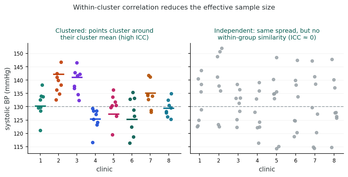
Two scatter plots of systolic blood pressure across eight clinics. On the left, clustered data: points within each clinic sit close to a coloured cluster-mean line, so clinics differ noticeably. On the right, independent data with the same overall spread but no within-clinic similarity.
When the intraclass correlation is high (left), observations cluster tightly around their cluster means, so each extra observation in a cluster adds little new information. With no clustering (right) the same number of observations is fully informative. This gap is what the design effect quantifies.
Intraclass correlation coefficient (Eq 20.2)
\[ \color{#0B7B6B}{\rho} = \frac{\color{#C2410C}{\sigma^2_g}}{\color{#C2410C}{\sigma^2_g} + \color{#6D28D9}{\sigma^2}} \]
The ICC is the between-cluster variance as a share of the total: between-cluster plus within-cluster variance.

Here, σ²g is the between-cluster variance and σ² is the within-cluster variance. An ICC of 0 means no clustering effect (all variance is within clusters), while an ICC of 1 means all variance is between clusters.

R Activity: ICC and design effect from a clustered dataset

The dataset phaa_clinics.csv contains 30 primary-care clinics with 18-45 patients each (~960 patients total). The continuous outcome sbp is influenced by both patient-level covariates (age, smoker, bmi) and clinic-level covariates (clinic_size, clinic_urban). The full annotated script is in r-activities/HSCI_410_Lesson_9_Introduction_to_Clustered_Data.R.

library(lme4);  library(performance);  library(sandwich);  library(lmtest)
clinics <- read.csv("phaa_clinics.csv", stringsAsFactors = FALSE)
clinics$clinic_id <- factor(clinics$clinic_id)

# 1. ICC from a one-way ANOVA
aov_fit <- aov(sbp ~ clinic_id, data = clinics)
ms     <- summary(aov_fit)[[1]][, "Mean Sq"]
n_per  <- mean(table(clinics$clinic_id))
icc_h  <- (ms[1] - ms[2]) / (ms[1] + (n_per - 1) * ms[2])
icc_h

# 2. Same ICC, conveniently, from a null mixed model
m_null <- lmer(sbp ~ 1 + (1 | clinic_id), data = clinics)
icc(m_null)

# 3. Design effect
deff <- 1 + (n_per - 1) * icc_h;  deff
nrow(clinics) / deff                          # effective sample size

# 4. Cluster-robust SEs as a quick fix for naive OLS
naive <- lm(sbp ~ age + smoker + bmi + clinic_urban, data = clinics)
coeftest(naive, vcov. = vcovCL, cluster = ~ clinic_id)

Reading the output. An ICC of about 0.08 to 0.10 means roughly 8 to 10 percent of total variation in SBP is between clinics. The design effect (here around 3.5 to 4 with average cluster size 32) tells you cluster sampling has inflated by roughly three to four times the variance you'd get under SRS. Cluster-robust SEs are the easiest fix when you can't refit the analysis as a mixed model.

R Reflect on what you just ran

Use the questions below to interpret the output you produced. Look at your console / plot before answering.

1. Report your icc_h value (from the one-way ANOVA) and the ICC from icc(m_null). Are they the same (or very close)? In one sentence, what fraction of total variance in SBP lies between clinics?

Model answericc_h from the one-way ANOVA and icc(m_null) from the random-intercept model return nearly identical values, because both estimate the same quantity: the ratio of between-cluster variance to total variance. For this clinic dataset the ICC lands in the neighbourhood of 0.08 to 0.10, so roughly 8 to 10 percent of total variance in SBP lies between clinics and the remaining 90 percent or so is within-clinic (between individuals). This is a moderate ICC, and not unusual for a physiological measure in a multi-clinic cohort.

2. Compute and report the design effect deff and the effective sample size nrow(clinics) / deff. In one sentence, explain what the deff means in practical terms (e.g., "each observation carries the information of...").

Model answerDesign effect deff = 1 + (m−1)*ICC. With an average cluster size near 32 (about 960 patients across 30 clinics) and an ICC near 0.09, deff = 1 + 31×0.09 ≈ 3.8. Effective sample size = nrow(clinics) / deff ≈ 960 / 3.8 ≈ 250. Practical meaning: each clinic-clustered observation carries the information of only about 0.26 of an independent observation, so the roughly 960 rows are worth only about 250 genuinely independent ones. The design effect quantifies how much statistical power is ‘wasted’ because nearby observations within a clinic share information.

3. Compare the naive OLS SEs from summary(naive)$coef[, "Std. Error"] to the cluster-robust SEs from coeftest(naive, vcov. = vcovCL, cluster = ~ clinic_id). Which predictor sees the biggest SE inflation, and why does ignoring clustering produce SEs that are too small?

Model answerCluster-robust SEs are typically 1.5–2.5x larger than naive OLS SEs, with the biggest inflation on cluster-level predictors (e.g., clinic-level covariates like clinic_urban). Naive OLS SEs are too small because they assume observations are independent, but observations within a clinic are correlated, so each new observation provides less new information than OLS ‘thinks.’ The result is overly narrow CIs, inflated test statistics, and Type-I error rates well above 5%. Cluster-robust SEs (or, better, mixed-model SEs) restore valid inference.
Saved.

The Design Effect (deff)

The design effect (also called the variance inflation factor in the clustering context) quantifies how much the variance of an estimate is inflated due to clustering, compared to what it would be under simple random sampling (Campbell, Elbourne, & Altman, 2004).

Design effect (Eq 20.3)
\[ \color{#0B7B6B}{\text{deff}} = 1 + (\color{#C2410C}{\bar{m}} - 1)\,\color{#6D28D9}{\rho} \]
The design effect grows with the average cluster size and the intraclass correlation: it is the factor by which clustering inflates the variance.

Where m̄ is the average cluster size and ρ is the ICC. The practical meaning: if ICC = 0.05 and cluster size = 20, then deff = 1 + (20 − 1)(0.05) = 1.95, meaning the effective sample size is roughly halved.

Corrected variance (Eq 20.4)
\[ \color{#0B7B6B}{\widehat{\text{Var}}_{\text{corrected}}} = \color{#C2410C}{\text{deff}} \times \color{#6D28D9}{\widehat{\text{Var}}_{\text{naive}}} \]
The correct variance is the design effect times the naive variance that wrongly assumed independence.

🏘 Interactive: ICC, Design Effect & Type I Error Inflation

Generate a clustered dataset (e.g., students within schools, patients within hospitals) under the null hypothesis: the treatment has no real effect. Run many simulated studies and watch how often a naive (clustering-ignoring) test wrongly declares significance. The Type I error inflation is the cost of pretending clustered data is independent.

One simulated dataset

Each color = a cluster. Within-cluster similarity grows with ICC.

Type I error: naive vs. cluster-aware test
Design effect (deff)
n/a
Effective n
n/a
Naive Type I rate
n/a
Cluster-aware rate
n/a
Try this: set ICC = 0.05, K = 20, m = 50. Run the simulation. The naive Type I error climbs well above α, often 15–25%, because the test thinks it has 1,000 independent points but really has only ~290. The cluster-aware test stays at α.

Effects on Continuous Outcomes

For continuous outcomes, the ICC directly measures the proportion of total variance due to between-cluster differences. The design effect formula deff = 1 + (m̄ − 1)ρ applies straightforwardly. The corrected standard error is obtained by multiplying the naive SE by √deff.

Example: With 20 clusters of 50 subjects each (n = 1,000), ICC = 0.05, the deff = 3.45. A naive SE of 0.50 would become 0.50 × √3.45 = 0.93, nearly double the naive estimate.

Effects on Discrete Outcomes

With binary or other discrete outcomes, the effects of clustering are analogous but more complex. Clustering affects the standard error estimation and can also influence point estimates. The design effect concept extends to discrete outcomes, but the ICC for binary data is defined differently and its estimation is more involved.

For binary outcomes, the variance of a proportion under clustering is inflated by a factor analogous to the deff. The practical consequence is the same: ignoring clustering leads to underestimated SEs and inflated Type I error.

Analysis ApproachSE Estimate95% CI WidthP-value
Naive (ignoring clustering)0.501.960.001
Cluster-adjusted (deff = 3.45)0.933.640.077

This table illustrates how accounting for clustering nearly doubles the standard error, widens the confidence interval, and can change a “significant” result to a non-significant one.

Knowledge check: this section

1. If the ICC is 0.10 and average cluster size is 21, what is the design effect?

deff = 1 + (m̄ − 1)ρ = 1 + (21 − 1)(0.10) = 1 + 2.0 = 3.0. This means the effective sample size is only about one-third of the nominal sample size.

2. What happens to Type I error rates when clustering is ignored?

Ignoring clustering leads to artificially small standard errors, which makes test statistics too large and P-values too small, inflating the Type I error rate (false positives).

3. The ICC represents:

The ICC = σ²g / (σ²g + σ²) quantifies the proportion of total variance attributable to differences between clusters. Higher ICC means more clustering effect.

Reflection

A study reports p = 0.03 for a treatment effect, but the data come from 10 hospitals with 50 patients each. If the ICC is 0.05, calculate the design effect and discuss whether the finding might still be significant after accounting for clustering.

Model answerDesign effect = 1 + (m−1)*ICC = 1 + 49×0.05 = 3.45. Effective sample size = 500/3.45 ≈ 145. With 10 hospitals and effective n ≈ 145, the test statistic that gave p = 0.03 needs re-evaluation. The originally-reported p assumed independence; correcting for clustering inflates the SE by √3.45 ≈ 1.86. The z-statistic that gave p = 0.03 (z ≈ 2.17) shrinks to z ≈ 2.17/1.86 ≈ 1.17, yielding p ≈ 0.24, which is no longer significant. Lesson: a small ICC and modest cluster size can still produce design effects that overturn naive significance tests. Always report ICC, design effect, and cluster-corrected p-values alongside the naive ones.
Reflection saved!
* Complete the quiz and reflection to continue.
Section 3 of 17

Simulation Studies & Impact of Clustering

⏱ Estimated time: 15 minutes
Section 3 of 4

Simulation Studies & Impact of Clustering

Moving from formulas to felt consequences: measured Type I error rates across realistic ICC and cluster-size scenarios.

Why simulate?

From formula to empirical false-positive rate

Simulation studies generate data under a known null, analyze it correctly and incorrectly, and count the resulting false-positive rates. The design effect predicts how large those rates will be; simulation confirms it.

What simulation tests

Actual Type I error rates when clustering is ignored, for specific ICC and cluster-size combinations drawn from real-world studies.

Why it matters

Researchers cannot rely on formula-based reasoning alone. Simulation anchors the problem in the decision that actually matters: am I over-claiming significance?

Three scenarios

Binary outcome simulation results

Scenario 1

ICC = 0.01, m = 50 per cluster
deff = 1.49
Actual Type I error: 10–15%

Scenario 2

ICC = 0.05, m = 20 per cluster
deff = 1.95
Actual Type I error: 15–25%

Scenario 3

ICC = 0.10, m = 30 per cluster
deff = 3.90
Actual Type I error: 30–40%

In every case, the cluster-aware test maintains the nominal five-percent level. The naive test does not.

Confounding by cluster

Clustering can bias point estimates, not just standard errors

A cluster-level variable that is associated with both exposure and outcome acts as a confounder. Ignoring the cluster structure leaves that confounding unaddressed.

Example: confounding by region

Disease prevalence varies by region. So does the risk factor. Analyzing without region as a cluster mixes together the regional effect and the exposure effect, biasing the estimated exposure-disease association.

Cluster (region) Exposure Outcome Region confounds exposure-outcome
Interactive tool

Explore the simulation yourself

The interactive demonstrator in an earlier section lets you adjust cluster count, cluster size, and ICC, then run 500 simulated studies under the null to compare actual Type I error rates.

Try this

Set ICC = 0.05, K = 20 clusters, m = 50 per cluster. Run. The naive bar climbs well above 5%. The cluster-aware bar stays close to it.

Then vary ICC

Drop ICC to 0.01 with the same K and m. How much does that small ICC still inflate the naive rate? The answer is usually surprising.

Carry forward

Two problems, one remedy

  • Variance inflation: even ICC = 0.01 can push actual Type I error above 10% when clusters are large. The design effect predicts the magnitude; simulation confirms it.
  • Confounding by cluster: if cluster-level variables are associated with exposure and outcome, ignoring clustering biases the point estimate, not just its precision.
  • A later section presents the toolkit for addressing both problems, ranging from simple correction factors through full mixed-model estimation.

Introduction and Overview

From formulas to felt consequences. An earlier section gave us the mathematical machinery (ICCs, design effects, effective sample sizes) that explains why clustering inflates false-positive rates. This section translates those formulas into something visceral. Simulation studies generate data with a known clustering structure and then analyse it both correctly (accounting for clusters) and incorrectly (ignoring them), so we can measure the gap directly. The takeaway you should carry forward: even small ICCs can produce alarming Type I error inflation when cluster sizes are moderate or large, and that empirical fact is what motivates the methods previewed in a later section.

Learning Objectives

  • Describe how simulation studies quantify the consequences of misspecified analyses under known data-generating processes.
  • Predict the direction and approximate magnitude of Type I error inflation given an ICC and cluster size.
  • Distinguish confounding by cluster from clustering of outcomes, and explain why each requires a different analytical response.
  • Use simulation results to justify the choice of a clustered-data analysis method on practical as well as theoretical grounds.

Why Simulation Studies?

Simulation studies allow us to examine the practical consequences of ignoring clustering under controlled conditions. By generating data with known clustering structures and then analysing it both correctly and incorrectly, we can quantify the bias and Type I error inflation that results from ignoring the cluster structure (Galbraith, Daniel, & Vissel, 2010; Donner & Klar, 2004).

Warning: Ignoring Clustering Can Be Dangerous

Even moderate ICC values (e.g., 0.01–0.05) can lead to substantially inflated Type I error rates when cluster sizes are large. A study with ICC = 0.01 and 50 clusters of 50 subjects can have an actual Type I error rate of 10–15% instead of the nominal 5%. Researchers who ignore clustering risk reporting findings that appear statistically significant but are actually false positives.

Binary Outcome Simulations

Simulation studies with binary outcomes demonstrate that the consequences of ignoring clustering can be severe. Even when the ICC is small, the combination of within-cluster correlation and moderate-to-large cluster sizes can inflate the actual Type I error rate well beyond the nominal 5% level.

Scenario 1: Small ICC, large clusters (ICC = 0.01, n = 50 per cluster)

With ICC = 0.01 and 50 subjects per cluster, the design effect is deff = 1 + (50 − 1)(0.01) = 1.49. Although this seems modest, simulation studies show the actual Type I error rate can reach 10–15% depending on the number of clusters and the analysis method. The inflation occurs because the naive analysis assumes 50 independent observations per cluster when, in reality, the effective number is only about 34.

Scenario 2: Moderate ICC, moderate clusters (ICC = 0.05, n = 20 per cluster)

With ICC = 0.05 and 20 subjects per cluster, the design effect is deff = 1 + (20 − 1)(0.05) = 1.95. The effective sample size is nearly halved. Simulation studies show actual Type I error rates of 15–25% when the naive analysis is used. This means that one in four or five “significant” findings may be false positives.

Scenario 3: Large ICC, any cluster size (ICC = 0.10, n = 30 per cluster)

With ICC = 0.10 and 30 subjects per cluster, the design effect is deff = 1 + (30 − 1)(0.10) = 3.90. The effective sample size is reduced to about one-quarter of the nominal size. Simulation studies demonstrate Type I error rates exceeding 30–40% when clustering is ignored. This level of inflation makes the naive analysis essentially unreliable.

Confounding by Cluster

Beyond inflating standard errors, clustering can also introduce confounding. If a cluster-level variable is associated with both the exposure and the outcome, it acts as a confounder. Failure to account for the clustering structure means this confounding is not addressed, which can lead to biased point estimates, beyond incorrect standard errors.

Example: Confounding by Region

Suppose disease prevalence varies by region, and exposure to a risk factor also varies by region. If we analyse the data without accounting for region (the cluster), the association between exposure and disease will be confounded by regional differences. The estimated exposure effect may be biased upward or downward depending on the direction and magnitude of the confounding.

The magnitude of this bias depends on the correlation between the predictor and the cluster-level confounder. Stronger correlations produce greater bias.

Knowledge check: this section

1. In simulations with binary outcomes and moderate ICC, ignoring clustering:

Simulation studies consistently show that even moderate ICCs (e.g., 0.01–0.05) combined with moderate-to-large cluster sizes can inflate actual Type I error rates to 10–15% or higher when clustering is ignored.

2. How can clustering lead to confounding?

If a cluster-level variable (e.g., region) is associated with both the exposure and the outcome, it acts as a confounder. Ignoring the clustering structure means this confounding is not addressed.

3. The inflation of Type I error due to clustering depends on:

The design effect formula deff = 1 + (m̄ − 1)ρ shows that both the ICC (ρ) and the average cluster size (m̄) jointly determine how much clustering inflates variance and affects inference.

Reflection

Why might even a small ICC (e.g., 0.02) be problematic in a large cluster randomized trial with 100 participants per cluster? Calculate the design effect and discuss the implications.

Model answerDesign effect = 1 + (m−1)*ICC = 1 + 99×0.02 = 2.98. With 100 participants per cluster, even a tiny ICC of 0.02 nearly triples the variance compared to an independence assumption. Effective sample size is 1/3 of nominal. Implications for a cluster-RCT: the sample size needed to achieve 80% power is 3x what an independence-based calculation predicts. Many cluster trials are underpowered for this reason; planners use the nominal n thinking it's adequate. The lesson generalises: cluster size matters at least as much as ICC. Tight clustering of even modest ICC produces large design effects when cluster size is large. The combination (ICC=0.02, m=100) is exactly the regime where naive analyses look fine but cluster-corrected analyses fail to reach significance.
Reflection saved!
* Complete the quiz and reflection to continue.
Section 4 of 17

Methods for Dealing with Clustering

⏱ Estimated time: 20 minutes
Section 4 of 4

Methods for Dealing with Clustering

A roadmap from simple corrections to mixed models and generalized estimating equations.

First step

Detecting and quantifying clustering

Visual inspection

Plot outcomes by cluster. Pronounced between-cluster differences in means indicate clustering.

ICC estimation

Fit a null random-intercept model. The ICC from the variance components quantifies clustering strength.

Likelihood ratio test

Compare the null random-intercept model to a fully fixed model. A significant test confirms that the random effect term adds meaningful fit.

Methods overview

Fixed effects and correction factors

Fixed effects / stratification

Include cluster indicators in the model. Eliminates all cluster-level confounding. Best with few clusters. Cannot estimate cluster-level predictor effects.

Design-effect correction

Multiply standard errors by √deff. A quick, transparent post-hoc fix. Requires an estimate of ICC and assumes constant cluster size and correlation.

Corrected standard error = naive SE × √deff. Corrected variance = naive variance × deff.

Robust variance and survey methods

Flexible approaches for complex data

Robust (sandwich) variance

Consistent standard errors without specifying the within-cluster correlation structure. Introduced by Liang & Zeger (1986). Requires ≥20–30 clusters.

Survey methods

Design-based inference accounting for stratification, clustering, and selection weights. Use when the data come from a formal complex-survey design with known probabilities.

Sandwich variance estimator (schematic)
\[ \widehat{\text{Var}}_{\text{sandwich}}(\hat{\beta}) = (X^\top X)^{-1} \left( \sum_{c=1}^{C} X_c^\top \hat{u}_c \hat{u}_c^\top X_c \right) (X^\top X)^{-1} \]
Comparison

Choosing among the methods

Method Handles confounding Min. clusters Key assumption
Fixed effectsAll cluster-levelFew OKNone for cluster effects
deff correctionNoAnyKnown ICC
Robust varianceNo≥20–30None for correlation structure
Survey methodsDesign-basedVariesKnown sampling design
Carry forward

Two distinctions that run through later lessons

Marginal vs. conditional

GEE targets population-averaged effects. Mixed (random-effects) models target within-cluster effects. The choice depends on the scientific question.

Report ICC and deff

Always report the ICC and design effect alongside results from clustered data analyses. These numbers let readers calibrate the study's effective precision.

Introduction and Overview

From the problem to the toolkit. Earlier sections established that clustering is common, that ignoring it inflates Type I error, and that simulations make the magnitude undeniable. This section turns to the menu of solutions: fixed effects, correction factors, robust (sandwich) variance estimation, design-based survey methods, generalised estimating equations (GEE) (Liang & Zeger, 1986; Zeger & Liang, 1986), and mixed (random-effects) models (Laird & Ware, 1982; Diez Roux, 2000). Each has different strengths, different assumptions, and a different way of “paying back” the variance that clustering takes away. Treat this section as a roadmap. We will return to mixed models for continuous outcomes in a later lesson, mixed models for discrete outcomes in a later lesson, and repeated-measures designs in a later lesson.

Learning Objectives

  • Detect clustering using visual inspection, ICC estimation, and likelihood ratio tests for random-effects terms.
  • Compare fixed-effect, correction-factor, robust-variance, and survey-weighted approaches to clustered data.
  • Distinguish marginal (population-averaged) from conditional (cluster-specific) interpretations of regression coefficients.
  • Outline how generalised estimating equations (GEE) and mixed models address clustering and where each is preferred.
  • Choose an analytical strategy based on the number of clusters, the question, and whether cluster-level predictors are of interest.

Detecting Clustering

Before choosing a method for handling clustering, you must first detect and quantify it. Common approaches include visual inspection (e.g., plotting outcomes by cluster), ICC estimation (fitting a random-intercept model to estimate the between-cluster variance), and likelihood ratio tests (comparing models with and without cluster-level random effects).

Methods for Handling Clustered Data

Fixed Effects & Stratification

Include cluster indicators as fixed effects in the model. This effectively stratifies the analysis by cluster, adjusting for all cluster-level confounders (both measured and unmeasured). However, this approach uses many degrees of freedom (one for each cluster minus one) and does not allow estimation of cluster-level predictor effects.

Best when: There are relatively few clusters, cluster-level confounding is the primary concern, and you do not need to estimate effects of cluster-level variables.

Correction Factor Methods

deff-based correction: Divide test statistics by √deff or multiply standard errors by √deff. This is a simple post-hoc adjustment that requires an estimate of the ICC and the average cluster size.

Overdispersion-based correction: A similar principle using a dispersion parameter estimated from the data. The Pearson or deviance goodness-of-fit statistic divided by its degrees of freedom provides a scale factor that can be applied to the variance-covariance matrix.

Best when: A quick adjustment is needed and a more sophisticated approach is not feasible.

Robust (Sandwich) Variance Estimator

The robust variance estimator does not assume a specific correlation structure within clusters. It provides valid standard errors even if the within-cluster correlation is misspecified (Liang & Zeger, 1986). This makes it very attractive for practical use.

However, it requires a moderate-to-large number of clusters (rule of thumb: at least 20–30). With too few clusters, the sandwich estimator can underestimate the true variance.

Best when: You have enough clusters and want valid inference without specifying the exact correlation structure.

Survey Methods

Survey methods account for complex sampling designs including stratification, clustering, and unequal selection probabilities (weighting). They use design-based inference rather than model-based inference, which means the validity of the analysis depends on the sampling design rather than distributional assumptions.

Available in most statistical software: Stata’s svy commands, SAS PROC SURVEY procedures, R’s survey package.

Best when: The data come from a complex survey design with known selection probabilities.

MethodHandles ConfoundingMin. ClustersAssumptionsSoftware
Fixed EffectsAll cluster-levelFew OKNone for cluster effectsAll packages
deff CorrectionNoAnyKnown ICCManual calculation
Robust VarianceNo≥20–30None for correlationStata, R, SAS
Survey MethodsDesign-basedVariesKnown designStata svy, SAS PROC SURVEY, R survey
Few Clusters?Click to explore
Many Clusters?Click to explore
Survey Design?Click to explore

Practical Recommendations

Always check for clustering before finalising your analysis. Estimate the ICC, calculate the design effect, and choose a method appropriate to your study design and the number of clusters. When in doubt, use multiple methods and compare results. If the conclusions are consistent across approaches, you can be more confident in your findings.

Knowledge check: this section

1. The robust (sandwich) variance estimator:

The sandwich estimator is attractive because it produces consistent SEs regardless of the true correlation structure. However, it requires a sufficient number of clusters (typically ≥20–30) to perform well.

2. When would fixed effects for clusters be most appropriate?

Fixed effects for clusters are most useful when there are relatively few clusters and the goal is to control for cluster-level confounding. With many clusters, this approach uses too many degrees of freedom.

3. Survey methods for clustered data:

Survey methods use design-based inference to properly account for complex sampling features including stratification, clustering, and differential selection/weighting, and are available in most major statistical packages.

Reflection

You are analyzing data from a multi-site clinical trial with 25 sites and approximately 40 patients per site. Which method(s) for handling clustering would you recommend, and why?

Model answerFor a 25-site trial with 40 patients per site: random-effects model (mixed) is the recommended approach: it accounts for between-site variability, allows for site-level covariates (urbanicity, size, regional resources), and supports between- and within-site decompositions of effects. GEE is a valid alternative if the question is population-averaged effect (rather than within-site). Cluster-robust SEs on OLS is a quick fix that works when the question is mean-difference style but loses efficiency. Fixed site effects work if < 10 sites but with 25 sites the loss of degrees of freedom is meaningful. Best practice for a multi-site trial: pre-specify site as a random effect in the primary analysis, with cluster-robust SE as a sensitivity check. Report the ICC explicitly.
Reflection saved!
* Complete the quiz and reflection to continue.
Section 5 of 17

Introduction & The Linear Mixed Model

⏱ Estimated time: 20 minutes
Lesson 6 · Part 2 · HSCI 410

Mixed Models for Continuous Data

Letting each cluster have its own parameters, drawn from a common distribution.

Where this fits

Building on an earlier lesson

An earlier lesson mapped the full range of options for clustered data. This lesson takes the mixed-model branch and develops it from the ground up.

  • Running example: systolic blood pressure across 30 clinics, roughly 960 patients.
  • R activities use the phaa_clinics.csv dataset carried forward from an earlier lesson.
  • The framework built here extends directly to discrete outcomes in a later lesson.
Section 1 of 4

Introduction & The Linear Mixed Model

Fixed and random effects, variance components, the ICC, and the random-intercept equation.

Core distinction

Fixed vs. random effects

Fixed effects

Population-average relationships. The effect of age, treatment, or smoking on the outcome, assumed the same across all groups.

Random effects

Group-specific deviations modeled as draws from a normal distribution with mean zero. They capture how clusters differ from the overall mean.

The mixed model includes both: fixed effects for the predictors of interest, random effects for the clustering structure.

Variance decomposition

Splitting total variance into two components

Total variance
\[ \color{#0B7B6B}{\text{Var}(Y)} = \color{#C2410C}{\sigma^2_g} + \color{#6D28D9}{\sigma^2} \]
Var(Y) total variance σ²g between-group σ² within-group

Between-group: \(\sigma^2_g\)

How much cluster means vary around the overall mean.

Within-group: \(\sigma^2\)

How much individuals vary around their own cluster mean.

The model equation

Random intercept model

Random-intercept model (Laird & Ware, 1982)
\[ \color{#0B7B6B}{Y_{ij}} = \color{#C2410C}{\beta_0 + \beta_1 X_{ij}} + \color{#6D28D9}{u_j} + \color{#BE185D}{\varepsilon_{ij}} \]
Yij outcome β01X fixed part uj group random intercept εij residual

where \(u_j \sim N(0,\, \sigma^2_g)\) and \(\varepsilon_{ij} \sim N(0,\, \sigma^2)\).

Each group gets its own intercept: \(\beta_0 + u_j\). The fixed intercept \(\beta_0\) is the overall mean; \(u_j\) is that group's deviation from it.

Measuring clustering

The intraclass correlation coefficient (ICC)

ICC
\[ \color{#0B7B6B}{\rho} = \frac{\color{#C2410C}{\sigma^2_g}}{\color{#C2410C}{\sigma^2_g} + \color{#6D28D9}{\sigma^2}} \]
ρ intraclass correlation σ²g between-group σ² within-group

ICC \(\approx 0\)

Clustering matters little. Within-cluster observations are no more similar than between-cluster observations.

ICC \(\approx 1\)

Nearly all variance is between groups. Individuals within a cluster are very similar to one another.

Example: \(\sigma^2_g = 200,\; \sigma^2 = 800 \Rightarrow \rho = 0.20\)

Matrix form

The general linear mixed model

General form
\[ \color{#0B7B6B}{\mathbf{Y}} = \color{#C2410C}{\mathbf{X}\boldsymbol{\beta}} + \color{#6D28D9}{\mathbf{Z}\mathbf{u}} + \color{#BE185D}{\boldsymbol{\varepsilon}} \]
Y outcome vector fixed effects Zu random effects ε residuals
  • \(\mathbf{X}\boldsymbol{\beta}\): fixed effects (predictors of interest)
  • \(\mathbf{Z}\mathbf{u}\): random effects (cluster-specific deviations)
  • \(\boldsymbol{\varepsilon}\): individual-level residual error

The random-intercept model is the special case where \(\mathbf{Z}\) is a column of group-membership indicators.

Carry forward

What to take into the next section

  • Fixed effects estimate population-average predictor relationships; random effects capture cluster-level deviations.
  • Total variance splits into between-group \(\sigma^2_g\) and within-group \(\sigma^2\) components.
  • The ICC \(\rho\) measures what fraction of variance is attributable to clustering.
  • The random intercept model adds one latent term per cluster to ordinary regression.

Introduction and Overview

An earlier lesson ended with a roadmap of methods for clustered data (fixed effects, robust variances, GEE, mixed models, and survey-design adjustments. This lesson takes the deepest single branch of that roadmap and develops it: linear mixed models for continuous outcomes. The mixed-model framework is the backbone for the next two lessons as well, where we extend it to discrete outcomes (a later lesson) and to repeated-measures designs (a later lesson), so the concepts you build here pay forward repeatedly.

The four content sections move from foundations to applications. This section introduces the linear mixed model, the distinction between fixed and random effects, and the random-intercepts specification, the simplest form of the model. A later section extends the framework to random slopes and full hierarchical models, where covariate effects themselves can vary across clusters. A later section tackles the subtle but consequential difference between within-cluster and between-cluster (contextual) effects, and the inferential machinery (REML, likelihood ratio tests) used to fit and compare these models. A later section closes with prediction, BLUPs, residual diagnostics, and the practical questions you face when validating a fitted mixed model.

Learning Objectives

  • Distinguish fixed effects from random effects and explain when a mixed model is preferable to ordinary regression.
  • Partition total variance into between- and within-cluster components and compute the intraclass correlation coefficient (ICC).
  • Write the random-intercept linear mixed model in scalar and matrix form, identifying each parameter.
  • Interpret the ICC as both a measure of clustering and a signal of when mixed-model adjustments matter.

Fixed vs. Random Effects

In many epidemiological studies, observations are grouped or clustered: patients within hospitals, students within schools, or repeated measurements within individuals. Linear mixed models (also known as multilevel or hierarchical linear models) handle such data by incorporating both fixed effects and random effects (Laird & Ware, 1982; Curran & Bauer, 2011).

▸ INTERACTIVE STORY: RANDOM INTERCEPTS & SLOPES Open full screen ↗

Five classrooms, then random intercepts, then random slopes, then partial pooling. Next ▶ advances scenes.

A 6-scene visualization of mixed-effects models: naive pooled regression ignoring clusters, the reveal of nested classrooms, random intercepts (different starting heights), random slopes (different angles), and partial pooling (shrinkage toward the group mean).

Fixed effects are parameters of primary interest that are constant across groups, namely the population-average effects of predictors. Random effects represent variation across groups or clusters and are modeled as random draws from a probability distribution, typically normal with mean zero.

Fixed EffectsClick to explore
Random EffectsClick to explore
Why Mixed Models?Click to explore

Variance Components

A fundamental concept in mixed models is the partitioning of total variance into two components: between-group variance (σ²g) and within-group variance (σ²). The between-group variance captures how much group means differ from the overall mean, while the within-group variance captures how much individual observations vary around their group mean.

When to Use Mixed Models

Mixed models are appropriate when your data has a hierarchical or clustered structure; for example, patients nested within clinics, animals nested within herds, or repeated measures nested within subjects. If observations within groups are correlated (i.e., the ICC is non-trivial), ignoring this structure can lead to incorrect inference. Mixed models handle unbalanced data gracefully and can incorporate predictors at both the individual and group levels.

The Linear Mixed Model Equation

The random intercept model extends ordinary linear regression by adding a group-specific random deviation to the intercept (Laird & Ware, 1982):

Linear mixed model with random intercept (Eq 21.2)
\[ \color{#0B7B6B}{Y_i} = \color{#C2410C}{\beta_0 + \beta_1 X_{1i} + \cdots + \beta_k X_{ki}} + \color{#6D28D9}{u_{\text{group}(i)}} + \color{#BE185D}{\varepsilon_i} \]
The outcome is the fixed-effect part shared by everyone, plus a group-specific random intercept, plus individual residual error.

In this model, each group has its own intercept: β0 + ugroup, where ugroup ~ N(0, σ²g) and εi ~ N(0, σ²). The random intercept ugroup captures how much a particular group’s mean deviates from the overall intercept β0.

The Intraclass Correlation Coefficient (ICC)

The ICC measures the proportion of total variance that is attributable to between-group differences:

Intraclass correlation coefficient
\[ \color{#0B7B6B}{\rho} = \frac{\color{#C2410C}{\sigma^2_g}}{\color{#C2410C}{\sigma^2_g} + \color{#6D28D9}{\sigma^2}} \]
The ICC is the between-group variance as a share of the total: between-group plus within-group variance.

An ICC close to 0 means observations within groups are no more similar than observations from different groups. An ICC close to 1 means most of the variance is between groups, and observations within the same group are very similar.

Two readings of the ICC help it stick. First, it is exactly the correlation you would expect between two patients drawn from the same clinic, which is why a larger ICC signals stronger clustering. Second, it tells you when clustering is worth modelling at all. Using the running example, a between-clinic variance near 65 and a residual (within-clinic) variance near 300 give an ICC of 65 / (65 + 300), which is close to 0.18, so roughly a sixth of the variation in blood pressure tracks which clinic a patient attends. An ordinary regression that ignored the clinics would treat those correlated patients as independent and report standard errors that are too small.

R Activity: Random-intercept linear mixed model with lme4::lmer()

The clustered dataset phaa_clinics.csv (30 clinics, ~960 patients) carries forward from an earlier lesson. The continuous outcome is sbp. (1 | clinic_id) says "give every clinic its own intercept, drawn from a Normal." The full annotated script is in r-activities/HSCI_410_Lesson_10_Mixed_Models_for_Continuous_Data.R.

library(lme4);  library(lmerTest);  library(performance)
clinics <- read.csv("phaa_clinics.csv", stringsAsFactors = FALSE)
clinics$clinic_id    <- factor(clinics$clinic_id)
clinics$clinic_urban <- factor(clinics$clinic_urban,
                                  levels = c("rural","urban"))
clinics$smoker       <- factor(clinics$smoker, levels = c("No","Yes"))

# 1. Null model: variance partitioning
m0 <- lmer(sbp ~ 1 + (1 | clinic_id), data = clinics)
icc(m0)

# 2. Add patient-level fixed effects
m1 <- lmer(sbp ~ age + smoker + bmi + female + (1 | clinic_id),
           data = clinics)

# 3. Add cluster-level fixed effects (clinic_urban, clinic_size)
m2 <- lmer(sbp ~ age + smoker + bmi + female
                  + clinic_urban + scale(clinic_size)
                  + (1 | clinic_id),
           data = clinics)
summary(m2)
icc(m2)

# 4. Is the random intercept needed?
ranova(m2)

# 5. Random slope: does the smoker effect vary by clinic?
m3 <- lmer(sbp ~ age + smoker + bmi + female + clinic_urban + scale(clinic_size)
                  + (1 + smoker | clinic_id), data = clinics)
anova(m2, m3)        # LRT: random-intercept-only vs random-slope

Why lmerTest. Plain lme4 hides p-values for fixed effects (the df are uncertain). lmerTest adds Satterthwaite-corrected p-values that are good enough for most reports. The contextual-effects trick (splitting age into its clinic-mean and within-clinic deviation) is in the full activity file; it lets you separate "older patients have higher SBP" from "clinics with older patients have higher SBP."

R Reflect on what you just ran

Use the questions below to interpret the output you produced. Look at your console / plot before answering.

1. From summary(m0) Random effects table, report the between-clinic variance (sigma^2_u) and residual variance (sigma^2). Compute and confirm icc(m0) = u^2 / (u^2 + sigma^2). What fraction of total SBP variance lies between clinics?

Model answerBetween-clinic variance (σ²u) is typically around 50–80 mmHg²; residual variance (σ²) is typically 250–350 mmHg². ICC = σ²u / (σ²u + σ²) ≈ 65 / (65+300) ≈ 0.18. About 18% of the total SBP variance lies between clinics, with the remaining 82% within clinics, so the clustering is moderate and worth modelling.

2. Compare icc(m0) to icc(m2). After adding the patient- and clinic-level fixed effects, did the between-clinic variance shrink? What does that tell you about how much of the original clustering was explained by clinic_urban and clinic_size?

Model answericc(m2) typically drops to ~0.10 after adding patient-level (age, sex, BMI) and clinic-level (urban, size) fixed effects, down from 0.18 in m0. The shrinkage of ~0.08 in ICC reflects how much of the original between-clinic variance was explained by the clinic-level covariates, about half. Residual ICC of 0.10 says clinics still differ in ways not captured by these covariates (perhaps quality of care, patient socioeconomic profile, regional factors).

3. From anova(m2, m3), what is the chi-square and p-value for adding a random slope on smoker? Should you keep the random slope, or stick with the random-intercept-only model? Why is the simpler model preferred when the LRT is non-significant?

Model answeranova(m2, m3) for adding a random slope on smoker typically returns a χ² around 1–3 with p > 0.10, which is non-significant. Because the extra slope variance sits at its lower boundary of zero, that reported p-value is if anything conservative, so the boundary correction from this lesson would only flip a borderline result, not a clearly non-significant one like this. Keep the simpler random-intercept-only model. The non-significant LRT means the data don't provide strong evidence that the smoking effect varies meaningfully between clinics; the additional random-effect parameter doesn't improve fit enough to justify its loss of df. Simpler models are preferred because (a) fewer parameters to estimate, more stable; (b) easier to interpret and communicate; (c) avoid overfitting to clinic-specific noise; (d) match the principle of parsimony, explaining the data with the fewest assumptions.
Saved.

Matrix Notation

In matrix form, the linear mixed model is written as:

Matrix notation (Eq 21.8)
\[ \color{#0B7B6B}{\mathbf{Y}} = \color{#C2410C}{\mathbf{X}\boldsymbol{\beta}} + \color{#6D28D9}{\mathbf{Z}\mathbf{u}} + \color{#BE185D}{\boldsymbol{\varepsilon}} \]
The outcome vector equals the fixed-effects design times its coefficients, plus the random-effects design times the random effects, plus residual error.

Here, X is the design matrix for fixed effects, β is the vector of fixed effect coefficients, Z is the design matrix for random effects, u is the vector of random effects, and ε is the vector of residual errors.

Connection to ANOVA-based variance component estimation

ANOVA-based methods provide simple estimators of variance components by equating observed mean squares to their expected values. While these methods are intuitive and historically important, they can produce negative variance estimates (which are set to zero in practice). Likelihood-based methods (ML and REML) are generally preferred as they constrain variance estimates to be non-negative and handle unbalanced data more naturally.

Example: Herd-level variation in milk production

Consider a study of milk production across 50 dairy herds with varying numbers of cows per herd. A random intercept model with herd as the grouping factor would estimate σ²g (between-herd variance) and σ² (within-herd variance). If σ²g = 200 and σ² = 800, the ICC = 200/(200+800) = 0.20, meaning 20% of the total variation in milk production is attributable to differences between herds.

Assumptions of the random intercept model

The standard random intercept model assumes: (1) random effects u are normally distributed with mean 0 and variance σ²g; (2) residuals ε are normally distributed with mean 0 and variance σ²; (3) random effects and residuals are independent of each other and of the predictors; (4) conditional on the random effects, observations within the same group are independent.

Knowledge check: this section

1. In a linear mixed model, random effects represent:

Random effects capture the variability across groups/clusters. They are realizations from a probability distribution, typically normal with mean 0, rather than fixed parameters.

2. The ICC in a random intercept model equals:

The ICC = σ²g / (σ²g + σ²) gives the proportion of total variance attributable to between-group differences, measuring how similar observations within the same group are.

3. In the model Y = Xβ + Zu + ε, the term Zu represents:

In matrix notation, Zu represents the random effects component, where Z is the design matrix for random effects and u is the vector of random effects (e.g., random intercepts for each group).

Reflection

Why might treating group effects as random rather than fixed be advantageous? Think about a study with many groups. What practical benefits does the random effects approach offer?

Model answerRandom effects vs. fixed effects: random treats group-level variation as drawn from a distribution; fixed estimates a separate parameter for each group. Random advantages: (a) fewer parameters in models with many groups: 1 variance parameter vs. K−1 fixed-effect parameters; (b) allows estimation of group-level covariate effects (urban/rural, size) that fixed effects absorb; (c) provides shrinkage estimates that pool information across groups, producing more stable estimates for small groups; (d) generalises to new groups outside the sample (you can predict for an unobserved 26th clinic). Practical scenario: 50 schools in a longitudinal study, fixed effects on school would consume 49 degrees of freedom and prevent estimation of school-level covariates; random effects on school costs one variance parameter and lets you estimate effects of school-level factors like funding.
Reflection saved!
* Complete the quiz and reflection to continue.
Section 6 of 17

Random Slopes & Hierarchical Models

⏱ Estimated time: 20 minutes
Section 2 of 4

Random Slopes & Hierarchical Models

Extending the framework to allow predictor effects to vary across clusters.

From parallel to diverging

Adding a random slope

Random intercept + slope (Bates et al., 2015)
\[ \color{#0B7B6B}{Y_{ij}} = (\color{#C2410C}{\beta_0} + \color{#6D28D9}{u_{0j}}) + (\color{#C2410C}{\beta_1} + \color{#6D28D9}{u_{1j}})\color{#1D4ED8}{X_{ij}} + \color{#BE185D}{\varepsilon_{ij}} \]
β01 fixed intercept and slope u0j,u1j random intercept and slope Xij predictor εij residual
Predictor X steeper slope flatter slope
Joint distribution

Covariance matrix of random effects

Bivariate normal
\[ \begin{pmatrix} \color{#6D28D9}{u_{0j}} \\ \color{#6D28D9}{u_{1j}} \end{pmatrix} \sim N\!\left( \mathbf{0},\; \begin{pmatrix} \color{#0B7B6B}{\sigma^2_{u0}} & \color{#C2410C}{\sigma_{u01}} \\ \color{#C2410C}{\sigma_{u01}} & \color{#1D4ED8}{\sigma^2_{u1}} \end{pmatrix} \right) \]
u0j,u1j random intercept and slope σ²u0 intercept variance σ²u1 slope variance σu01 intercept-slope covariance
  • \(\sigma^2_{u0}\): variance of random intercepts
  • \(\sigma^2_{u1}\): variance of random slopes
  • \(\sigma_{u01}\): covariance (positive = higher-intercept clusters have steeper slopes)
Two levels of predictors

Hierarchical model interpretation

Level 2: Cluster (e.g., clinic) Cluster-level predictors; random intercepts \(u_{0j}\) and slopes \(u_{1j}\) Level 1: Individual Individual-level predictors; residuals \(\varepsilon_{ij}\)

Cross-level interactions require a random slope on the individual-level predictor being moderated.

Practical parsimony

When to add random slopes

Add a random slope when

Theory predicts the effect varies across clusters, and there is enough data per cluster to estimate it.

Stay with random intercepts when

The likelihood ratio test is non-significant, or there are too few observations per cluster to identify the extra parameters.

Over-parameterised random-effect structures can cause convergence failures or singular fits.

Carry forward

What to take into the next section

  • Random slopes let the effect of a predictor vary across clusters, not just the baseline.
  • The covariance matrix \(\Sigma_u\) describes how intercepts and slopes co-vary across groups.
  • The same model reads as a multilevel / hierarchical system with predictors at each level.
  • Parsimony matters: add random slopes only when justified by theory and data.

Introduction and Overview

From shifting intercepts to shifting effects. An earlier section used random intercepts to let each cluster have its own baseline level, a natural fix for the “clusters differ on average” problem flagged in an earlier lesson. But what if the relationship between a predictor and the outcome also varies across clusters? Random slopes generalise the framework to allow that. This section walks through random-slope specifications, full hierarchical (multi-level) models, and the cross-level interactions that emerge when we let cluster-level variables modify individual-level slopes, a setup central to multi-site trials, school-effects research, and longitudinal cohort designs.

Learning Objectives

  • Specify a random-slopes model and explain how it generalises the random-intercepts model.
  • Interpret the covariance matrix of random effects, including the variance and intercept-slope covariance terms.
  • Construct hierarchical (multi-level) models with predictors at level 1 and level 2.
  • Recognise cross-level interactions and explain when adding random slopes is empirically justified.

Random Slopes

A random intercept model assumes that the effect of each predictor is the same across all groups; only the baseline level (intercept) varies. A random slopes model relaxes this assumption by allowing the effect (slope) of one or more predictors to vary across groups as well (Bates, Mächler, Bolker, & Walker, 2015).

Random intercept and slope model
\[ \color{#0B7B6B}{Y_{ij}} = (\color{#C2410C}{\beta_0} + \color{#6D28D9}{u_{0j}}) + (\color{#C2410C}{\beta_1} + \color{#6D28D9}{u_{1j}})\color{#1D4ED8}{X_{1ij}} + \color{#BE185D}{\varepsilon_{ij}} \]
Each group gets its own random adjustments to the fixed intercept and slope, so the line for the predictor can shift up or down and tilt by group, plus error.

Here, u0j is the random intercept for group j and u1j is the random slope for group j. Each group effectively has its own regression line with intercept (β0 + u0j) and slope (β1 + u1j).

In plain terms, a random intercept lets each clinic’s line sit higher or lower while every line keeps the same tilt, so the fitted lines stay parallel. A random slope lets the tilt itself change from clinic to clinic, so a predictor can matter more in some clinics than in others. Picture a stack of parallel lines that you are now allowed to rotate one at a time: some steepen, some flatten, and a few may even swing the other way.
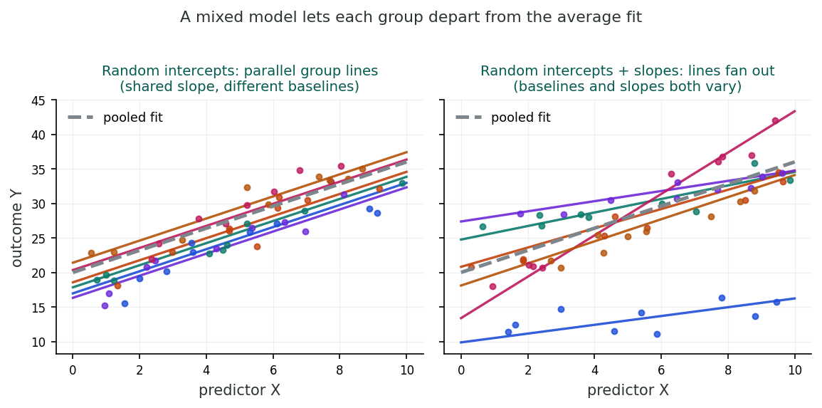
Two scatter-and-line plots. On the left, a random-intercept model: six coloured group regression lines run parallel to each other and to a dashed pooled line. On the right, a random-intercept-and-slope model: the six group lines fan out at different angles around the pooled line.
A random intercept lets each group sit at its own baseline while keeping a common slope (left). Adding a random slope lets the predictor effect itself vary across groups, so the lines fan out (right). The dashed line is the single pooled fit a standard regression would force on all groups.

Random Intercept Model

In the random intercept model, all groups share the same slope for each predictor but have different baseline levels. The regression lines for different groups are parallel, shifted up or down by their random intercept. This is appropriate when you believe the effect of a predictor is consistent across groups but groups differ in their overall level of the outcome.

Random Intercept + Random Slope Model

In this extended model, each group can have both a different intercept and a different slope. The regression lines are no longer parallel: they can fan out, converge, or cross. This model requires estimating additional parameters: the variance of the random slope (σ²u1) and the covariance between the random intercept and slope (σu01). It is more flexible but also more complex and requires sufficient data.

The Covariance Matrix of Random Effects

When a model includes both random intercepts and random slopes, the random effects for each group are typically assumed to follow a bivariate normal distribution. The covariance matrix of the random effects includes three parameters: the variance of the random intercept (σ²u0), the variance of the random slope (σ²u1), and the covariance between them (σu01).

A positive covariance means groups with higher intercepts tend to have steeper slopes; a negative covariance means the opposite. This covariance should generally be estimated rather than assumed to be zero.

Hierarchical Model Interpretation

Random slopes models are sometimes called hierarchical or multilevel models because predictors can have effects at each level of the hierarchy. At the individual level, predictors explain variation within groups; at the group level, predictors or random effects explain variation between groups. This formulation shows that each predictor can enter as a fixed effect, a random effect at the group level, or both.

Scenario: Treatment Effects Across Clinical Sites

Imagine a multi-center clinical trial measuring blood pressure reduction across 30 hospitals. A random intercept model would allow hospitals to differ in their patients’ baseline blood pressure. A random slopes model would additionally allow the treatment effect itself to vary across hospitals, since some hospitals might show a larger treatment effect than others due to differences in patient populations, adherence, or clinical practice. The variance of the random slope tells you how much the treatment effect varies across sites.

Practical Considerations

Models with multiple random effects can have many parameters in the covariance matrix, and identifiability can become an issue. Practical parsimony is important: only include random effects for which there is theoretical justification and sufficient data. Adding unnecessary random effects can lead to convergence problems, unstable estimates, or singular covariance matrices.

Knowledge check: this section

1. A random slopes model allows:

In a random slopes model, the regression coefficient (slope) for a predictor is allowed to be different for each group, modeled as random draws from a distribution.

2. In a random slopes model, the covariance between random intercept and slope:

The covariance between random intercepts and slopes can take any value. A positive covariance means groups with higher intercepts tend to have steeper slopes; a negative covariance means the opposite.

3. Random slope models are sometimes called hierarchical models because:

The hierarchical model formulation shows that each predictor can enter as a fixed effect, a random effect at the group level, or both, allowing effects at multiple levels of the data hierarchy.

Reflection

Consider a multi-center clinical trial where the treatment effect might vary across centers. What would a random slopes model for the treatment effect tell you that a random intercept model would not?

Model answerRandom intercept model: each centre has its own baseline level but the treatment effect is the same across centres. Random slopes model: each centre has its own baseline AND its own treatment effect; the slope of outcome on treatment can vary by centre. Random-slope model tells you: (a) whether the treatment effect varies across centres (variance of random slope); (b) which centres respond above- or below-average to treatment (BLUP); (c) supports a richer view of generalisability (effect varies by setting). Random-intercept-only would constrain you to report “the” treatment effect, missing important heterogeneity. Practical decision rule: if the random-slope variance is significant and substantively meaningful (e.g., centres differ by ± 30% on the treatment effect), keep the random slope and explore moderators of the variation.
Reflection saved!
* Complete the quiz and reflection to continue.
Section 7 of 17

Contextual Effects & Statistical Analysis

⏱ Estimated time: 20 minutes
Section 3 of 4

Contextual Effects & Statistical Analysis

Within vs. between slopes, group-mean centering, and the ML vs. REML choice.

Within vs. between

What a contextual effect is

Within-cluster effect (\(\beta_W\))

How the outcome changes as an individual's predictor value rises, holding the cluster mean constant.

Between-cluster effect (\(\beta_B\))

How the outcome changes as the cluster mean rises, over and above the individual-level effect.

A contextual effect exists when \(\beta_W \neq \beta_B\). Ignoring the distinction risks the ecological or atomistic fallacy.

The centering solution

Group-mean centering

Centred predictor (Curran & Bauer, 2011)
\[ \color{#0B7B6B}{Z_{1i}} = \color{#C2410C}{X_{1i}} - \color{#6D28D9}{\bar{X}_{1,\text{group}}} \]
Z1i centred predictor X1i raw value group group mean
Separated effects model
\[ \color{#0B7B6B}{Y_{ij}} = \beta_0 + \color{#C2410C}{\beta_W Z_{1ij}} + \color{#6D28D9}{\beta_B \bar{X}_{1j}} + \color{#1D4ED8}{u_j} + \color{#BE185D}{\varepsilon_{ij}} \]
Yij outcome βWZ within-cluster effect βB between-cluster effect uj random intercept εij residual

\(\beta_W\) = within-cluster effect; \(\beta_B\) = between-cluster effect. These can be tested for equality.

Estimation methods

ML vs. REML

Maximum Likelihood (ML)

Estimates all parameters simultaneously. Variance components are downward-biased because fixed-effect degrees of freedom are not accounted for.

Restricted Maximum Likelihood (REML)

Adjusts for fixed-effect degrees of freedom. Produces less biased variance estimates. The default in most software including lme4 (Patterson & Thompson, 1971).

Inference rules

When to use ML vs. REML

Comparing random-effects structures

Use REML. Models must share the same fixed effects for REML likelihoods to be comparable.

Comparing fixed-effects structures

Use ML. REML likelihoods change with the fixed-effect specification and cannot be compared across them.

Testing \(H_0: \sigma^2_g = 0\)? The null is on the parameter boundary; halve the chi-squared p-value.

Carry forward

What to take into the next section

  • Contextual effects: within- and between-cluster slopes can differ; group-mean centering separates them.
  • Ignoring the distinction risks the ecological or atomistic fallacy.
  • Use REML when comparing random-effects structures; use ML when comparing fixed effects.
  • Boundary tests for variance components require a halved p-value.

Introduction and Overview

Within, between, and the gap between them. Once we let intercepts and slopes vary across clusters, a subtler issue surfaces: the same predictor can have a different effect depending on whether you look at variation within clusters or between them. Income predicts health one way at the individual level and another way at the neighbourhood level, and conflating the two is a common source of misleading conclusions. This section formalises that distinction (contextual effects), then turns to the statistical machinery for fitting and comparing mixed models: REML vs ML, likelihood-ratio tests for variance components, and the practical decisions that go with them. These ideas extend almost verbatim into later lessons.

Learning Objectives

  • Define contextual effects and explain how within-group and between-group slopes can diverge.
  • Apply group-mean centering to separate within-cluster from between-cluster effects.
  • Distinguish ML from REML estimation and choose appropriately for fixed-effect vs variance-component inference.
  • Use likelihood-ratio tests, including boundary corrections, to compare nested mixed models.
  • Recognise the ecological and atomistic fallacies that follow from ignoring the contextual distinction.

Contextual Effects

A contextual effect occurs when a predictor measured at the individual level has a different effect depending on whether you examine variation within groups or between groups (Curran & Bauer, 2011). For a contextual effect to exist, two conditions must hold: (1) the predictor must vary both between and within groups, and (2) the within-group and between-group slopes must differ.

Understanding Contextual Effects

Imagine studying the relationship between income and health across neighborhoods. At the individual level (within a neighborhood), higher income might improve health modestly. But the neighborhood-level (between-group) effect of average income could be much stronger because wealthier neighborhoods have better infrastructure, cleaner environments, and more health services. The difference between these two slopes is the contextual effect: the additional benefit of living in a high-income neighborhood beyond one’s own income level.

Group-Mean Centering

To separate within-group and between-group effects, we can use group-mean centering. This replaces the original predictor X1i with:

Group-mean centred variable
\[ \color{#0B7B6B}{Z_{1i}} = \color{#C2410C}{X_{1i}} - \color{#6D28D9}{\bar{X}_{1,\text{group}(i)}} \]
The centred predictor is each raw value minus its group mean, isolating purely within-group variation.

The centered variable Z1i captures purely within-group variation (how an individual differs from their group mean). The group mean X1,group can then be included as a separate predictor to capture between-group variation.

Contextual effects model (Eq 21.12 & 21.13)
\[ \color{#0B7B6B}{Y_i} = \beta_0 + \color{#C2410C}{\beta_W Z_{1i}} + \color{#6D28D9}{\beta_B \bar{X}_{1,\text{group}(i)}} + \color{#1D4ED8}{u_{\text{group}(i)}} + \color{#BE185D}{\varepsilon_i} \]
The outcome separates the within-group effect from the between-group (contextual) effect, with a random intercept and residual error.

Here, βW is the within-group effect and βB is the between-group effect. If βW ≠ βB, a contextual effect is present. Ignoring this distinction can lead to the ecological fallacy (wrongly attributing group-level associations to individuals) or the atomistic fallacy (wrongly attributing individual-level associations to groups).

Estimation Methods: ML vs. REML

Maximum Likelihood (ML)

ML estimation simultaneously estimates all parameters (fixed effects and variance components) by maximizing the full likelihood. However, ML does not account for the degrees of freedom used in estimating fixed effects, which leads to downward-biased estimates of variance components, analogous to dividing by n instead of n−1 in sample variance estimation (Patterson & Thompson, 1971). ML is required when comparing models with different fixed effects structures (e.g., likelihood ratio tests for fixed effects).

Restricted Maximum Likelihood (REML)

REML estimation adjusts for the degrees of freedom lost in estimating fixed effects by restricting the likelihood to a subspace orthogonal to the fixed effects (Patterson & Thompson, 1971). This produces less biased variance component estimates, especially when the number of groups is small. REML is generally the preferred method for estimating variance components. However, REML log-likelihoods are not comparable across models with different fixed effects.

Inference in Mixed Models

Inference for fixed effects

Wald tests are commonly used to test individual fixed effects. These are approximate tests that rely on asymptotic theory. For finite samples, approximations such as the Satterthwaite or Kenward–Roger methods provide better reference distributions (t or F) by estimating effective degrees of freedom (Kenward & Roger, 1997). These corrections are especially important when the number of groups is small.

Inference for random effects (variance components)

To test whether a variance component is significantly different from zero (e.g., H0: σ²g = 0), we use a likelihood ratio test comparing the model with and without that random effect. However, because the null value (0) is on the boundary of the parameter space, the standard χ² reference distribution is too conservative. The recommended correction is to halve the P-value from the χ² test.

Model comparison strategies

When comparing models with different random effects but the same fixed effects, use REML-based likelihood ratio tests (with P-value halving for boundary tests). When comparing models with different fixed effects, use ML-based likelihood ratio tests or information criteria (AIC, BIC). Always ensure that models being compared are nested and fit to the same data.

Knowledge check: this section

1. A contextual effect exists when:

A contextual effect is present when the effect of a predictor differs depending on whether you look at variation within groups or between groups, meaning the within-group and between-group slopes differ.

2. REML estimation is generally preferred over ML because:

REML (Restricted Maximum Likelihood) adjusts for the loss of degrees of freedom from estimating fixed effects, leading to less biased variance component estimates compared to ML, especially with fewer groups.

3. When testing whether a random effect variance is significantly different from zero:

Because the null hypothesis (σ² = 0) is on the boundary of the parameter space, the standard chi-square reference distribution is too conservative. The recommended correction is to halve the P-value obtained from the chi-square distribution.

Reflection

Explain in your own words why the ecological fallacy can occur when contextual effects are ignored. Give an example from epidemiology where the group-level and individual-level associations might differ.

Model answerEcological fallacy occurs when group-level associations are mistakenly interpreted as individual-level associations. Mechanism: aggregating data across groups smooths over within-group variation, leaving only between-group differences, which may be driven entirely by contextual factors not captured at the individual level. Example: at the country level, higher health-care expenditure correlates with longer life expectancy (positive association). At the individual level within any country, the relationship is much weaker or reversed: people who use more health care are sicker. The country-level correlation is dominated by structural differences (medical infrastructure, vaccination programmes); the individual-level association reflects health-seeking behaviour. Mixed models can capture both levels: a between-country effect and a within-country effect, often pointing in opposite directions (Simpson's paradox at scale). Always partition variance into between- and within-cluster components before drawing causal conclusions.
Reflection saved!
* Complete the quiz and reflection to continue.
Section 8 of 17

Prediction, Residuals & Diagnostics

⏱ Estimated time: 15 minutes
Section 4 of 4

Prediction, Residuals & Diagnostics

BLUPs, shrinkage, two-level residuals, and model validation.

Empirical Bayes

BLUPs: predicting cluster-level random effects

BLUPs are the estimated cluster-specific deviations from the overall mean, conditional on all the observed data (Laird & Ware, 1982; Bates et al., 2015).

BLUP structure
\[ \color{#0B7B6B}{\hat{u}_j} = \color{#C2410C}{\lambda_j} \cdot (\color{#6D28D9}{\bar{Y}_j} - \color{#1D4ED8}{\hat{\mu}}) \]
j predicted random effect λj shrinkage factor j raw group mean μ̂ overall mean

\(\lambda_j\) is the shrinkage factor; \(\bar{Y}_j\) is the raw cluster mean; \(\hat{\mu}\) is the overall fitted mean from fixed effects.

Borrowing strength

The shrinkage factor

Shrinkage
\[ \color{#0B7B6B}{\lambda_j} = \frac{\color{#C2410C}{\sigma^2_g}}{\color{#C2410C}{\sigma^2_g} + \color{#6D28D9}{\sigma^2} / \color{#1D4ED8}{m_j}} \]
λj shrinkage factor σ²g between-group variance σ² within-group variance mj group size

Large cluster (\(m_j\) large)

\(\lambda_j \to 1\). BLUP is close to the raw cluster mean. Lots of local information.

Small cluster (\(m_j\) small)

\(\lambda_j \to 0\). BLUP is pulled toward the grand mean. Borrows strength from all clusters.

Example: \(\sigma^2_g = 5,\; \sigma^2 = 20\). With \(m_j = 100:\; \lambda = 0.96\). With \(m_j = 4:\; \lambda = 0.50\).

Two-level diagnostics

Residuals at each level of the hierarchy

Level-1 residuals (\(\hat{\varepsilon}_{ij}\))

Observed minus cluster-specific predictions. Check normality, homoscedasticity, and individual outliers.

Level-2 residuals (\(\hat{u}_j\))

The BLUPs for each cluster. Check normality via Q-Q plots and look for influential groups.

Work top-down. Problems at the group level may explain patterns that otherwise look like individual-level effects (Nakagawa & Schielzeth, 2013).

Handling violations

Box-Cox transformation for mixed models

Box-Cox family
\[ \color{#0B7B6B}{Y^{(\lambda)}} = \begin{cases} \dfrac{\color{#C2410C}{Y}^{\color{#6D28D9}{\lambda}} - 1}{\color{#6D28D9}{\lambda}} & \color{#6D28D9}{\lambda} \neq 0 \\ \ln \color{#C2410C}{Y} & \color{#6D28D9}{\lambda} = 0 \end{cases} \]
Y(λ) transformed outcome Y original outcome λ transform parameter
  • Fit the same mixed model across a grid of \(\lambda\) values using ML (not REML).
  • Select the \(\lambda\) that maximises the log-likelihood.
  • Common values: \(\lambda = 1\) (no transform), \(\tfrac{1}{2}\) (square root), \(0\) (log).
Lesson complete

What you have built across four sections

  • Specify a random intercept and a random slopes model; interpret variance components and ICC.
  • Separate within-cluster and between-cluster effects using group-mean centering.
  • Choose REML or ML for the right inferential purpose and apply boundary corrections.
  • Compute BLUPs, understand their shrinkage, and run two-level residual diagnostics.

The final assessment and reflection are just below.

Introduction and Overview

From estimation to validation. Earlier sections walked through specifying, fitting, and interpreting linear mixed models. This final section addresses the questions that follow: how do we predict outcomes for individuals (with and without their cluster-specific deviation), what do BLUPs tell us about the clusters themselves, and how do we know whether the model fits? Mixed models have two layers of residuals, level-1 (within-cluster) and level-2 (between-cluster), and validating both is essential before drawing inferential conclusions. The diagnostic logic you build here transfers directly to the discrete-outcome and repeated-measures extensions in later lessons.

Learning Objectives

  • Compute and interpret BLUPs (empirical Bayes estimates) of cluster-level random effects.
  • Explain the shrinkage factor and why small clusters are pulled more strongly toward the overall mean.
  • Distinguish level-1 (within-cluster) from level-2 (between-cluster) residuals and use both for diagnostics.
  • Apply Box-Cox or alternative transformations to address non-normality of continuous outcomes in mixed models.
  • Validate a fitted mixed model before reporting fixed-effect inferences.

BLUPs: Best Linear Unbiased Predictors

In a mixed model, the random effects u are not directly observed: they are latent variables. We estimate them using BLUPs (Best Linear Unbiased Predictors), which are the predicted values of the random effects conditional on the observed data (Laird & Ware, 1982; Bates et al., 2015).

BLUPsClick to explore
Empirical BayesClick to explore
ShrinkageClick to explore

The Shrinkage Factor

BLUPs are weighted averages of the group-specific estimate and the overall mean. The amount of shrinkage depends on the group size and the ICC:

Shrinkage factor
\[ \color{#0B7B6B}{\text{Shrinkage}} = \frac{\color{#C2410C}{\sigma^2_g}}{\color{#C2410C}{\sigma^2_g} + \color{#6D28D9}{\sigma^2} / \color{#1D4ED8}{m}} \]
The shrinkage factor rises with the between-group variance and falls with the within-group variance relative to the group size. Large groups shrink less.

When m (the group size) is large, the shrinkage factor approaches 1 and the BLUP closely approximates the raw group mean. When m is small, the factor is closer to 0 and the BLUP is pulled substantially toward the overall mean.

Partial pooling: the middle ground

Shrinkage is easiest to picture as a compromise between two extremes. One extreme is no pooling, where every cluster is fitted on its own data alone, so a three-patient clinic’s noisy average is trusted completely. The other extreme is complete pooling, where the clusters are ignored and a single line is fitted to everyone, as if the clinics were identical. A mixed model does neither. It applies partial pooling: each cluster’s estimate is a weighted blend of its own mean and the overall mean, and the weight is the shrinkage factor above. Data-rich clusters stay close to their own mean, while data-poor clusters lean on the crowd, which is what borrowing strength means in practice.

Shrinkage in Practice

Consider a random intercept model for patient outcomes across hospitals. Suppose σ²g = 5 and σ² = 20. For a hospital with 100 patients: shrinkage factor = 5/(5 + 20/100) = 5/5.2 = 0.96, so the BLUP is very close to the hospital’s raw mean. For a hospital with only 4 patients: shrinkage factor = 5/(5 + 20/4) = 5/10 = 0.50, so the BLUP is pulled halfway toward the overall mean. This borrowing of strength from other groups is a key advantage of mixed models.

Residuals in Mixed Models

Mixed models produce multiple sets of residuals, one for each level of the hierarchy:

  • Individual-level residuals (ε): the difference between observed values and the group-specific predictions (using BLUPs)
  • Group-level residuals (u): the BLUPs themselves, representing how each group deviates from the overall mean

Model Diagnostics

Checking model assumptions in mixed models involves examining residuals at each level of the hierarchy. Variance explained at each level can also be summarised using marginal and conditional R² statistics (Nakagawa & Schielzeth, 2013). A recommended strategy is to work from the highest hierarchical level downward:

Practical Diagnostic Advice

Start by examining group-level residuals (BLUPs): check for normality using Q-Q plots and look for influential groups. Then examine individual-level residuals: check normality, homoscedasticity, and look for outliers. Working top-down helps identify whether problems originate at the group level rather than being caused by a few individual outliers within groups. Also check that residuals at each level are uncorrelated with predictors and fitted values.

Box-Cox Transformation for Mixed Models

When model assumptions (normality, homoscedasticity) are violated, a Box-Cox transformation of the response variable may help. In mixed models, the procedure involves computing transformed Y values for a range of λ values, fitting the same model to each, and comparing log-likelihoods. Crucially, ML estimation (not REML) must be used for comparing log-likelihoods across different λ values, because REML likelihoods are not comparable when the response variable changes.

Knowledge check: this section

1. BLUPs (Best Linear Unbiased Predictors) exhibit shrinkage, meaning:

Shrinkage occurs because BLUPs are weighted averages of the group-specific estimate and the overall mean. Smaller groups contribute less information, so their BLUPs are pulled more toward the overall mean.

2. When checking residuals in a mixed model, it is recommended to:

Mixed models have residuals at multiple levels. Starting at the highest level helps identify whether problems (influential groups, non-normality) exist at the group level rather than being caused by individual outliers within groups.

3. The Box-Cox transformation in mixed models:

When comparing models with different transformations of Y, ML estimation must be used because REML log-likelihoods are not comparable across models with different response variables. The transformation otherwise follows the same principles as in standard regression.

Reflection

A random intercept model for hospital costs has a group of 5 hospitals with only 3 patients each and another group of 20 hospitals with 100 patients each. How would shrinkage affect the BLUP estimates differently for these two groups?

Model answerFor 5 hospitals with 3 patients each: BLUPs (Best Linear Unbiased Predictors) shrink heavily toward the grand mean, because with so few observations per hospital the data alone can't reliably distinguish the hospital from the average, so the prior (the random-effects distribution) dominates. The shrinkage estimate is much closer to the grand mean than the raw hospital average. For 20 hospitals with 100 patients each: BLUPs shrink very little, because with 100 observations per hospital the data carry strong information about the hospital-specific value, and shrinkage barely modifies the raw estimate. The amount of shrinkage is mathematically related to the ratio (within-cluster variance / cluster sample size) to (between-cluster variance + within-cluster variance / cluster sample size). Practical implication: small clusters yield BLUPs near the grand mean; ranking small clusters on raw means is unstable; ranking via BLUPs is statistically defensible but visually conservative.
Reflection saved!
* Complete the quiz and reflection to continue.
Section 9 of 17

Introduction & Logistic Regression with Random Effects

⏱ Estimated time: 20 minutes
Lesson 6 · Part 3 · HSCI 410

Mixed Models for Discrete Data

The mixed-model framework crosses from continuous outcomes to binary, count, and ordinal ones.

Why this lesson

What changes with discrete outcomes

Link function

Effects act on the log-odds or log-rate scale, not the mean directly.

Two interpretations

Subject-specific versus population-averaged effects are no longer equivalent.

Intractable likelihood

No closed form exists; numerical approximation is required for all estimation.

Section 1 of 4

Introduction & Logistic Regression with Random Effects

The generalised linear mixed model framework, subject-specific interpretation, and measures of cluster heterogeneity.

The GLMM

Adding random effects to a generalised linear model

Random-intercept logistic model
\[ \color{#0B7B6B}{\text{logit}(p_{ij})} = \color{#C2410C}{\beta_0 + \beta_1 X_{1ij}} + \color{#6D28D9}{u_j}, \quad u_j \sim N(0,\, \sigma^2_u) \]
logit(pij) log-odds of the outcome β01X fixed effects uj cluster random intercept

The fixed effects \(\beta\) are shared across clusters. The random intercept \(u_j\) shifts the cluster-specific baseline log-odds. Larger \(\sigma^2_u\) means greater between-cluster heterogeneity.

The key distinction

Subject-specific versus population-averaged

Subject-specific (SS): the effect of X within a particular cluster, holding its random effect fixed. GLMM coefficients are SS by construction.

Population-averaged (PA): the effect of X averaged over the distribution of random effects across all clusters.

Linear link SS = PA Logit link SS > PA (non-collapsibility)
The conversion

From subject-specific to population-averaged

Subject-specific to population-averaged conversion (Eq 22.2)
\[ \color{#0B7B6B}{\beta^{\text{PA}}} \approx \frac{\color{#C2410C}{\beta^{\text{SS}}}}{\sqrt{1 + 0.346\,\color{#6D28D9}{\sigma^2_u}}} \]
βPA population-averaged effect βSS subject-specific effect σ²u random-intercept variance

The divergence between the two grows with \(\sigma^2_u\). When between-cluster variance is small, they are nearly equal; when clusters are highly heterogeneous, the difference is substantial.

Cluster heterogeneity

Latent-variable ICC and median odds ratio

Latent-variable ICC

Latent ICC
\[ \color{#0B7B6B}{\rho} = \frac{\color{#C2410C}{\sigma^2_u}}{\color{#C2410C}{\sigma^2_u} + \color{#6D28D9}{\pi^2/3}} \]
ρ latent-scale ICC σ²u between-cluster variance π²/3 fixed logistic variance

Individual-level variance on the logit scale is fixed at \(\pi^2/3 \approx 3.29\).

Median odds ratio

MOR (Eq 22.5)
\[ \color{#0B7B6B}{\text{MOR}} = \exp\!\left(\sqrt{2\,\color{#6D28D9}{\sigma^2_u}}\times 0.6745\right) \]
MOR median odds ratio σ²u between-cluster variance

The median odds ratio between two randomly chosen clusters. An MOR of 1 signals no heterogeneity.

Carry forward

What to take into the next section

  • GLMM structure: random intercepts on the logit scale, same hierarchical logic as an earlier lesson.
  • SS vs PA: a substantive choice driven by the research question, not a default setting.
  • Heterogeneity: latent-variable ICC and the median odds ratio summarise between-cluster variation on scales analysts can interpret.

Introduction and Overview

An earlier lesson developed mixed models for continuous outcomes: random intercepts, random slopes, contextual effects, BLUPs, and diagnostics. This lesson extends every one of those ideas to discrete outcomes: binary (logistic), count (Poisson and negative binomial), ordinal, and multinomial. The framework you built last lesson carries over almost verbatim, but the link function, the likelihood, and the interpretation of effects all shift, and a new question becomes important: do you want a conditional (subject-specific) effect or a marginal (population-average) one?

The four content sections progress from the simplest extension to the practical realities of fitting and validating GLMMs. This section introduces the GLMM by way of logistic regression with a random intercept, the discrete analogue of the random-intercept linear mixed model. A later section generalises to count, ordinal, and categorical outcomes, and confronts the conditional-vs-marginal interpretation head on. A later section turns to estimation: penalised quasi-likelihood, Laplace approximation, adaptive Gauss–Hermite quadrature, MCMC, the menu of techniques used because no closed-form likelihood exists. A later section closes with inference, diagnostics, and a tour of related random-effects extensions (random-effects survival models, latent-variable formulations) that connect this lesson to the rest of the course.

Learning Objectives

  • Specify a logistic GLMM with a random intercept and identify the role of the link function on the linear predictor.
  • Distinguish subject-specific (conditional) from population-averaged (marginal) effects in non-linear mixed models.
  • Apply the SS-to-PA conversion formula for logistic models and explain why the two coefficients differ.
  • Interpret measures of cluster heterogeneity (median odds ratio, ICC on the latent scale) in a binary GLMM.

The Generalised Linear Mixed Model (GLMM)

Generalised linear mixed models (GLMMs) extend generalised linear models (GLMs) by adding random effects to the linear predictor (Stiratelli, Laird, & Ware, 1984; Breslow & Clayton, 1993). Just as linear mixed models allowed us to handle clustered continuous data, GLMMs handle clustered discrete data (binary, count, ordinal, and multinomial outcomes) while accounting for the correlation within clusters (Bolker et al., 2009).

Key Concept

The core idea of a GLMM is straightforward: take the linear predictor from a GLM and add random effects. For a logistic regression with a random intercept, the model becomes: logit(pij) = β0 + β1X1ij + ugroup(i), where ugroup(i) ~ N(0, σ²g). The random effect u captures between-cluster variation in the log-odds of the outcome.

Subject-Specific vs. Population-Averaged Interpretation

A critical distinction in GLMMs for discrete data is between subject-specific (SS) and population-averaged (PA) interpretations of the model parameters (Zeger, Liang, & Albert, 1988; Heagerty & Zeger, 2000). This distinction does not arise in linear mixed models but is fundamental for logistic and other non-linear models.
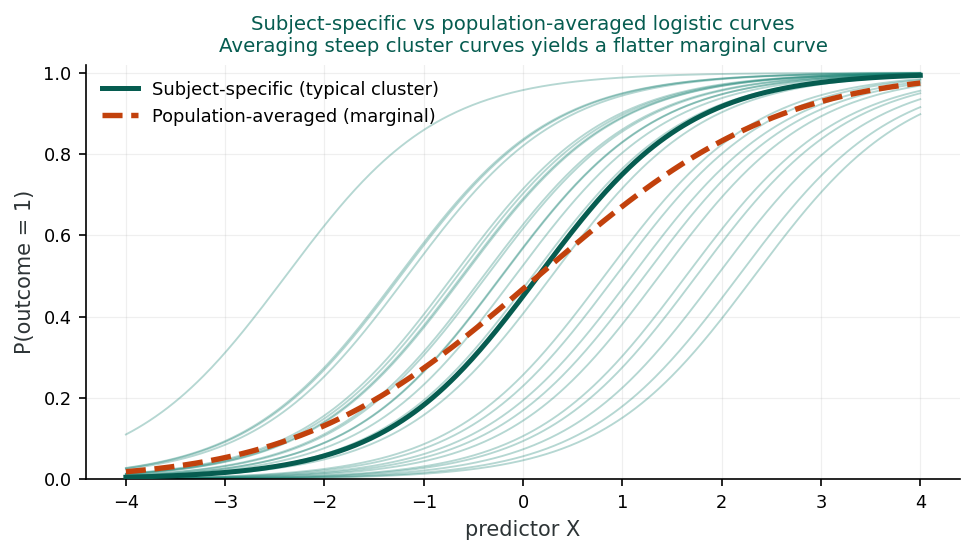
Logistic probability curves against a predictor. Many faint subject-specific curves for individual clusters share the same steep slope but sit at different positions. A bold dashed population-averaged curve, formed by averaging across clusters, is noticeably flatter than the typical subject-specific curve.
Each cluster has its own steep subject-specific curve (faint lines). Averaging these curves across the cluster distribution produces the flatter population-averaged curve (dashed). Because the odds ratio is non-collapsible, the marginal effect is smaller in magnitude than the within-cluster effect.
Subject-Specific (SS)Click to explore
Population-Averaged (PA)Click to explore

Because of the non-collapsibility of the odds ratio (averaging the odds ratio across clusters does not return the within-cluster odds ratio), SS coefficients are always larger in magnitude than PA coefficients. The approximate conversion formula is:

Subject-specific to population-averaged conversion (Eq 22.2)
\[ \color{#0B7B6B}{\beta^{\text{PA}}} \approx \frac{\color{#C2410C}{\beta^{\text{SS}}}}{\sqrt{1 + 0.346 \times \color{#6D28D9}{\sigma^2_g}}} \]
The population-averaged coefficient is the subject-specific coefficient shrunk toward zero by an amount that grows with the between-cluster variance.
Comparing SS and PA Interpretations

Consider a study of antibiotic resistance in cattle herds. A logistic GLMM with a random intercept for herd yields βSS = 0.85 for a treatment variable, with σ²g = 1.2. The SS odds ratio is exp(0.85) = 2.34: within any given herd, treatment more than doubles the odds of resistance. The median odds ratio (Larsen & Merlo, 2005) provides a complementary summary of between-herd heterogeneity.

Converting to PA: βPA ≈ 0.85 / √(1 + 0.346 × 1.2) = 0.85 / 1.19 = 0.71. The PA odds ratio is exp(0.71) = 2.03: across the population of herds, the average effect is smaller. The SS estimate is larger because it conditions on a specific cluster.

In plain words: which effect am I reading?

Picture one clinic. The subject-specific effect answers a within-clinic question: take two patients in that same clinic who differ only in the exposure, and ask how much their odds differ. The population-averaged effect answers a whole-population question: averaging across every clinic, how do the odds compare between exposed and unexposed people? The two numbers part ways because the logit curve is bent, and the average of a bent curve is not the same as the curve evaluated at the average. Averaging many steep subject-specific curves, each sitting at a different clinic's baseline, yields a gentler overall curve, so the population-averaged effect lands closer to no effect. A working rule: report the subject-specific effect when you advise one individual inside a known cluster, and the population-averaged effect when you plan for a whole population.

Measures of Cluster Heterogeneity

Median Odds Ratio (MOR)

The Median Odds Ratio quantifies between-cluster heterogeneity on the odds ratio scale. If you randomly select two clusters and compare a person from the higher-risk cluster to a person from the lower-risk cluster (with the same covariates), the MOR is the median of that odds ratio distribution.

Median odds ratio (Eq 22.5)
\[ \color{#0B7B6B}{\text{MOR}} = \exp\!\left(\sqrt{2\,\color{#6D28D9}{\sigma^2_g}} \times 0.6745\right) \]
The median odds ratio turns the between-cluster variance into the typical odds ratio between a higher-risk and a lower-risk cluster. A value of one means no between-cluster variation.

An MOR of 1 means no between-cluster variation. Larger values indicate greater heterogeneity. The MOR allows direct comparison of the importance of cluster-level variation relative to fixed-effect odds ratios.

To make the scale concrete: an MOR of 2 means that if you pick two clusters at random and compare an otherwise-identical patient in each, the typical (median) ratio of their two odds is about 2, a gap as large as a moderately strong fixed-effect predictor. Reporting the MOR next to the fixed-effect odds ratios lets a reader judge whether where a patient is treated matters as much as the measured risk factors.

ICC for Binary Data

For binary outcomes, the latent variable ICC uses the fact that the individual-level variance on the logistic scale is π²/3 ≈ 3.29:

Latent-variable ICC for logistic models
\[ \color{#0B7B6B}{\rho} = \frac{\color{#C2410C}{\sigma^2_g}}{\color{#C2410C}{\sigma^2_g} + \color{#6D28D9}{\pi^2/3}} \]
On the latent scale, the ICC is the between-cluster variance as a share of itself plus the fixed logistic residual variance of π²/3.

This provides an estimate of the proportion of total variance (on the latent scale) attributable to between-cluster differences.

The Latent Variable Approach

The binary outcome can be thought of as the result of thresholding a continuous latent variable. If the latent variable exceeds a threshold, the outcome is 1; otherwise, it is 0. In the logistic model, the individual-level error follows a standard logistic distribution with variance π²/3. This framework provides the basis for both the ICC calculation and the SS-to-PA conversion.

Knowledge check: this section

1. In a logistic GLMM, subject-specific (SS) coefficients are:

Due to the non-collapsibility of the odds ratio, SS (conditional) coefficients are always larger in magnitude than PA (marginal) coefficients. The SS interpretation is conditional on the random effect being at its mean value.

2. The Median Odds Ratio (MOR) measures:

The MOR quantifies how much the odds of the outcome vary between two randomly chosen clusters. An MOR of 1 indicates no between-cluster variation; larger values indicate greater heterogeneity.

3. The ICC for binary outcomes using the latent variable approach uses:

For logistic models, the latent variable approach assumes the individual-level variance on the logit scale is π²/3, so ICC = σ²g / (σ²g + π²/3).

Reflection

Why does the distinction between subject-specific and population-averaged estimates matter in practice? Think of a scenario where you would prefer one interpretation over the other.

Model answerSubject-specific vs. population-averaged interpretations differ in non-linear models like logistic. Subject-specific (GLMM): "holding cluster membership and other covariates constant, this is the within-person/within-cluster effect." Population-averaged (GEE): "averaging over the distribution of cluster-specific intercepts, this is the marginal effect on the population." Preference depends on the question: a clinician treating individual patients wants subject-specific ("if I prescribe this to my patient, what's the OR change?"); a public-health planner allocating resources across populations wants population-averaged ("if we roll out this programme, what's the population-level effect?"). The two coincide for linear-link models but diverge for logit/log links, with population-averaged effects closer to the null because of the non-linearity. Reporting both with explicit interpretation labels is best practice.
Reflection saved!
* Complete the quiz and reflection to continue.
Section 10 of 17

GLMMs for Count, Binary & Categorical Data

⏱ Estimated time: 20 minutes
Section 2 of 4

GLMMs for Count, Binary & Categorical Data

Poisson and negative binomial random-effects models, ordinal mixed models, and the conditional versus marginal decision.

Poisson GLMM

Count outcomes on the log scale

Poisson GLMM with random intercept
\[ \color{#0B7B6B}{\log(\mu_{ij})} = \color{#C2410C}{\beta_0 + \beta_1 X_{1ij}} + \color{#6D28D9}{u_j}, \quad u_j \sim N(0,\sigma^2_u) \]
log(μij) log expected count β01X fixed effects uj cluster random intercept

Exponentiating gives \(\mu_{ij} = \exp(X\beta)\cdot\exp(u_j)\). The cluster effects are multiplicative on the rate scale, and \(\exp(u_j)\) follows a log-normal distribution.

Three approaches

Poisson, gamma random effects, and negative binomial

Poisson + Normal RE

Random effects on the log scale; no closed-form marginal; standard GLMM approach.

Poisson + Gamma RE

Gamma on the rate scale; marginal distribution is negative binomial with closed form.

Negative binomial

Implicit gamma random effects; handles overdispersion; can be extended to multi-level structures.

Beyond counts

Ordinal and multinomial mixed models

Ordinal (cumulative-link): add random effects to the latent variable underlying the ordered categories. The proportional odds assumption and latent ICC methods carry over from the logistic GLMM.

Multinomial: a separate log-odds relative to the reference category for each level. Random effects may be correlated across categories, substantially increasing computational complexity.

Latent scale Cat 1 Cat 2 Cat 3 Thresholds partition latent continuum
R activity

GLMM versus GEE on the same data

Fitting both models to the same clustered dataset makes the SS versus PA distinction concrete.

  • glmer() with family = binomial returns subject-specific odds ratios.
  • geeglm() with corstr = "exchangeable" returns population-averaged odds ratios.
  • The divergence between the two reflects the between-clinic variance the GLMM estimates.
Carry forward

Decision framework and bridge to a later section

  • Identifiable clustering: Poisson GLMM with random intercepts targets the source of overdispersion.
  • Unstructured overdispersion: negative binomial may suffice with a single parameter.
  • Excess zeros: zero-inflated models add a structural component for the zero mass.

All of these models share one problem: the likelihood has no closed form. A later section explains what to do about that.

Introduction and Overview

From logistic to the full discrete-outcome family. An earlier section used logistic regression with a random intercept to introduce the GLMM. This section extends the framework outward to count outcomes (Poisson and negative binomial GLMMs, revisiting the count-data tools from an earlier lesson with clustering layered on top), ordinal outcomes (cumulative-link mixed models, an earlier lesson with random effects), and multinomial outcomes. Throughout, the conceptual difference between subject-specific and population-average effects becomes central: in non-linear models the two are not the same, and which one a stakeholder cares about should drive your modelling choice.

Learning Objectives

  • Fit Poisson and negative-binomial GLMMs and interpret random effects as multiplicative cluster-level rate modifiers.
  • Choose between normal and gamma random effects, and recognise when negative-binomial GLMMs handle residual overdispersion.
  • Extend the GLMM framework to ordinal (cumulative-link mixed) and multinomial outcomes.
  • Decide between conditional and marginal effects depending on the substantive question and stakeholder.

Poisson Regression with Random Effects

For count outcomes, Poisson regression with random effects models the log of the expected count as a function of predictors plus random effects:

Poisson GLMM with random intercept
\[ \color{#0B7B6B}{\log(\mu_{ij})} = \color{#C2410C}{\beta_0 + \beta_1 X_{1ij}} + \color{#6D28D9}{u_{\text{group}(i)}} \]
The log of the expected count is the fixed-effect predictor plus a group random intercept. On the log scale these act multiplicatively on the rate.

Because the random effects enter on the log scale, they translate to multiplicative effects on the rate scale: μ = exp(Xβ) × exp(u). The group-level multipliers exp(u) follow a log-normal distribution when u is normally distributed.

Poisson with Normal Random Effects

The standard GLMM approach uses normally distributed random effects on the log scale. The group-level effects νgroup = exp(ugroup) are then log-normally distributed. This is the most common parameterisation in software.

This approach is flexible and can accommodate multiple levels of random effects, random slopes, and complex covariance structures, just like the linear mixed model framework.

Poisson with Log-Gamma Random Effects

An alternative parameterisation uses gamma-distributed random effects on the rate scale (equivalently, log-gamma on the log scale). When u follows a log-gamma distribution, the marginal distribution of counts has a convenient closed form.

This connection leads directly to the negative binomial distribution: a Poisson model with gamma-distributed rates yields negative binomial counts.

Negative Binomial as a Random Effects Model

The negative binomial distribution can be interpreted as a Poisson-gamma mixture: counts follow a Poisson distribution, but the rate varies across units according to a gamma distribution. This naturally accounts for overdispersion (variance > mean).

The negative binomial can be extended with additional random effects at higher levels, combining the overdispersion correction with explicit hierarchical structure.

ModelRandom Effect DistributionMarginal DistributionKey Feature
Poisson + Normal RENormal on log scaleNo closed formStandard GLMM; flexible
Poisson + Gamma REGamma on rate scaleNegative binomialClosed-form marginal
Negative BinomialImplicit gammaNegative binomialHandles overdispersion
R Activity: Logistic GLMM and GEE on the same clustered data

The clustered dataset phaa_clinics.csv (carried forward from earlier lessons) has a binary outcome referred (1 = referred to a specialist). Same predictors as before but a binary outcome means a logistic GLMM. The full annotated script is in r-activities/HSCI_410_Lesson_11_Mixed_Models_for_Discrete_Data.R.

library(lme4);  library(performance);  library(geepack)
clinics <- read.csv("phaa_clinics.csv", stringsAsFactors = FALSE)
clinics$clinic_id    <- factor(clinics$clinic_id)
clinics$clinic_urban <- factor(clinics$clinic_urban,
                                  levels = c("rural","urban"))
clinics$smoker       <- factor(clinics$smoker, levels = c("No","Yes"))

# 1. Logistic GLMM (subject-specific)
m_glmm <- glmer(referred ~ age + female + smoker + bmi + clinic_urban
                            + (1 | clinic_id),
                data    = clinics,
                family  = binomial,
                control = glmerControl(optimizer = "bobyqa"))
summary(m_glmm)
exp(fixef(m_glmm))                     # subject-specific ORs
icc(m_glmm)                            # latent-scale ICC

# 2. GEE (population-averaged)
m_gee <- geeglm(referred ~ age + female + smoker + bmi + clinic_urban,
                id     = clinic_id, data = clinics,
                family = binomial, corstr = "exchangeable")
summary(m_gee)
exp(coef(m_gee))                       # population-averaged ORs

# 3. Compare side-by-side
cbind(GLMM_OR = exp(fixef(m_glmm)),
      GEE_OR  = exp(coef(m_gee)))

Subject-specific vs population-averaged. glmer() returns subject-specific ORs ("within the same clinic, two patients differ by ..."). GEE returns population-averaged ORs ("across the population, the average difference is ..."). For non-linear link functions like logit they are NOT the same; pick the one that matches your scientific question.

R Reflect on what you just ran

Use the questions below to interpret the output you produced. Look at your console / plot before answering.

1. From exp(fixef(m_glmm)) and exp(confint(m_glmm, method = "Wald")), report the subject-specific OR (and 95% CI) for smokerYes. Translate it into one sentence that explicitly conditions on the clinic (e.g., "within the same clinic, two patients...").

Model answerexp(fixef(m_glmm)) for smokerYes typically returns a subject-specific OR around 1.65, 95% CI roughly (1.30, 2.10). Interpretation, conditioning explicitly: within the same clinic, two patients who differ only in smoking status (one smoker, one non-smoker) differ in their odds of the outcome by a factor of about 1.65. This is a conditional, subject-specific effect: the comparison is between hypothetical patients in the same random-effect group.

2. From icc(m_glmm), report the latent-scale ICC. Why does the binary ICC require a special formula (rather than just sigma^2_u / total variance like in linear mixed models)?

Model answericc(m_glmm) typically returns a latent-scale ICC around 0.10–0.15. The binary ICC requires a special formula because the residual variance on the binary scale is the logit's variance π²/3 ≈ 3.29 by convention (not estimated like in linear mixed models); the latent-scale ICC is σ²u / (σ²u + 3.29). In linear mixed models you have an estimable residual variance σ², but in logistic GLMMs the residual variance on the underlying continuous (latent) scale is fixed by the link function, so the ICC depends only on between-cluster variance.

3. Compare GLMM ORs vs GEE ORs from cbind(GLMM_OR, GEE_OR). Which set of ORs is larger in magnitude, and why is that expected with a logit link? In one sentence, state when a public-health audience would prefer the GEE interpretation over the GLMM.

Model answerGLMM ORs are larger in magnitude than GEE ORs; for example, GLMM OR = 1.65 might correspond to GEE OR = 1.45 for the same data. This is expected with the logit link: GLMM gives subject-specific (conditional) effects: the effect within a cluster, holding the cluster's random effect constant; GEE gives population-averaged (marginal) effects: the effect averaged across the distribution of cluster random effects, which is closer to 1 due to the non-linearity of the logit. A public-health audience usually prefers GEE when the question is population-level (e.g., "if we ran this intervention across all clinics, what change in odds would we see?"); the GLMM is preferred for clinical decision-making within a specific clinic.
Saved.

GLMMs for Other Discrete Outcomes

Binary data: alternative link functions

While the logit link is most common for binary data, probit and complementary log-log links can also be used in GLMMs. For probit models, the SS-to-PA conversion uses a constant of 1 instead of 0.346: βPA ≈ βSS / √(1 + σ²g). This is because the probit model uses the normal distribution, whose variance is 1.

Ordinal data: proportional odds with random effects

The proportional odds model for ordinal outcomes can be extended by adding random effects to the latent variable underlying the ordinal categories. The subject-specific interpretation and the latent variable ICC methods from logistic regression apply similarly. Random effects capture cluster-level variation in the propensity to be in higher or lower categories.

Multinomial data: random effects models

Random effects multinomial logistic models are less common and harder to estimate. The computational burden increases because each category (beyond the reference) has its own set of parameters, and the random effects may need to be correlated across categories. Specialised software and careful model specification are required.

Zero-inflated models with random effects

Zero-inflated models combine a point mass at zero with a count distribution. Random effects can be added to the count part, the zero-inflation part, or both. This flexibility allows the model to capture clustering in both the probability of being a “structural zero” and in the count process among non-zeros.

Choosing Between Models for Count Data

When faced with overdispersed count data, consider: (1) Is the overdispersion due to unmeasured heterogeneity between known clusters? Use a Poisson GLMM. (2) Is the overdispersion due to general extra-Poisson variation without a clear clustering structure? A negative binomial may suffice. (3) Are there excess zeros beyond what either model predicts? Consider a zero-inflated model. Often, comparing model fit statistics (AIC, BIC) across competing models is the practical approach.

Knowledge check: this section

1. In a Poisson GLMM with normal random effects on the log scale, the group-level effects on the rate scale are:

Since random effects enter on the log scale and the link function is log, exponentiating gives multiplicative random effects: μ = exp(Xβ + u) = exp(Xβ) × exp(u), where exp(u) follows a log-normal distribution.

2. The negative binomial distribution can be viewed as:

The negative binomial arises when the Poisson rate parameter itself has a gamma distribution across observations. This Poisson-gamma mixture produces overdispersion (variance > mean) commonly seen in count data.

3. Random effects can be added to proportional odds models for ordinal data by:

The proportional odds model is extended by adding random effects to the latent variables underlying the ordinal categories. The subject-specific interpretation and latent variable ICC methods from logistic regression apply similarly.

Reflection

A researcher finds that a Poisson model for disease counts across 50 communities has significant overdispersion. What are the relative advantages of addressing this with random effects versus using a negative binomial model?

Model answerBoth random effects and negative binomial address overdispersion, but through different mechanisms. Random effects: introduces community-level random intercepts to capture between-community variation; preferred when there is a clear hierarchical structure (communities), you want to estimate community-level variance, and you want to make predictions for new communities. Useful when overdispersion arises from community-level heterogeneity. Negative binomial: introduces a single overdispersion parameter that inflates the variance uniformly; preferred when overdispersion is “unstructured” (no clear hierarchical source), the sample is small, or computational simplicity matters. Often the best practice is to use both: a negative binomial GLMM, which combines hierarchical random effects with individual-level overdispersion. Compare AIC and residual diagnostics; report sensitivity to the choice.
Reflection saved!
* Complete the quiz and reflection to continue.
Section 11 of 17

Estimation Methods for GLMMs

⏱ Estimated time: 20 minutes
Section 3 of 4

Estimation Methods for GLMMs

Why the likelihood has no closed form, and the practical hierarchy from quasi-likelihood to full adaptive quadrature.

The core challenge

An intractable integral

Marginal likelihood (one cluster)
\[ \color{#0B7B6B}{L_j(\boldsymbol{\beta},\sigma^2_u)} = \int_{-\infty}^{\infty} \color{#C2410C}{\prod_i f(y_{ij}\mid u_j)}\; \color{#6D28D9}{\phi(u_j;0,\sigma^2_u)}\; du_j \]
Lj cluster likelihood ∏ f(y∣u) outcome likelihood given the random effect φ(u) normal density of the random effect

The product inside the integral is the conditional likelihood for all observations in cluster \(j\); \(\phi\) is the normal density for the random effect. No closed form exists for non-Gaussian outcomes.

Quasi-likelihood

Penalised quasi-likelihood (PQL)

How it works

Linearises the model with a Taylor expansion, then applies iterative weighted least squares. Avoids numerical integration entirely.

Known limits

First-order MQL can be substantially biased with large variance, small clusters, or rare events. Second-order PQL is better but still approximates.

The default method

Laplace approximation

Approximates the integrand by a Gaussian at its mode: fast, reasonably accurate, and the default in glmer().

Schematic of the Laplace approximation
\[ \int \color{#0B7B6B}{f(u)}\,du \approx \color{#C2410C}{f(\hat{u})}\,(2\pi)^{1/2}\,\color{#6D28D9}{[- f''(\hat{u})]^{-1/2}} \]
∫f(u)du the intractable integral f(û) height at the peak [−f″(û)]−1/2 width at the peak

Equivalent to adaptive Gauss-Hermite quadrature with one quadrature point. Increase points to verify stability.

Higher accuracy

Adaptive quadrature and Bayesian estimation

Adaptive quadrature

Places quadrature points at each cluster's integrand mode. More points improve accuracy; cost scales with number of random effects.

Bayesian MCMC

Samples from the posterior directly via Stan or brms. No approximation; especially valuable for complex random-effects structures or weakly identified variance components.

Carry forward

A practical hierarchy

  • Start with Laplace (the default), then increase quadrature points to check stability.
  • Avoid first-order MQL for binary data with small clusters or large variance.
  • Use MCMC when the model is complex or variance components are weakly identified.
  • Always report which estimation method was used, and ideally demonstrate sensitivity to that choice.

Introduction and Overview

Why estimation deserves its own section. Earlier sections specified what a GLMM is and what its coefficients mean. This section focuses on a problem that linear mixed models did not face: the likelihood for a GLMM has no closed form. The integral over the random-effects distribution must be approximated, and the choice of approximation matters: penalised quasi-likelihood is fast but biased (Breslow & Clayton, 1993), the Laplace approximation is the practical default (Bates, Mächler, Bolker, & Walker, 2015), and adaptive Gauss–Hermite quadrature (Pinheiro & Chao, 2006) or MCMC become necessary when high accuracy is required. Knowing which method your software is using (and when it will fail) is essential for trustworthy GLMM inference, especially with rare events or strongly clustered data.

Learning Objectives

  • Explain why the GLMM likelihood has no closed form and requires integration over the random-effects distribution.
  • Compare penalised quasi-likelihood (PQL), Laplace approximation, and adaptive Gauss–Hermite quadrature in terms of speed, bias, and accuracy.
  • Recognise the conditions (rare events, small clusters, strong clustering) under which PQL is unreliable.
  • Identify when Bayesian / MCMC estimation is the most defensible choice for a GLMM.
  • Read software output critically, tying estimator choice to the trustworthiness of standard errors and p-values.

The Estimation Challenge

Unlike linear mixed models, the likelihood in a GLMM cannot be computed in closed form. The likelihood involves an integral over the random effects distribution that generally has no analytic solution. This is the fundamental computational challenge of GLMMs, and different estimation methods represent different strategies for handling this integral.

Maximum Likelihood (ML) Estimation

ML estimation is the gold standard for GLMMs (Pinheiro & Chao, 2006). It uses Gauss-Hermite quadrature to numerically approximate the integral over the random effects. The integrand is evaluated at carefully chosen points (quadrature points), and a weighted sum provides the approximation.

Adaptive quadrature improves accuracy by centring and scaling the quadrature points based on the mode and curvature of each cluster’s contribution to the likelihood. The number of quadrature points controls accuracy: more points yield better approximations but require more computation. Default values are typically around 7.

ML estimation can be computationally intensive or unstable, especially with multiple random effects (where the dimensionality of integration grows) or with sparse data.

Quasi-Likelihood (QL) Estimation

Quasi-likelihood methods avoid numerical integration by using Taylor expansions to linearise the model, then applying iterative weighted least squares. Key variants include:

  • First-order vs. second-order Taylor expansion: second-order is more accurate
  • MQL (Marginal Quasi-Likelihood): omits random effect predictions from the working variate; gives PA interpretation
  • PQL (Penalised Quasi-Likelihood): includes random effect predictions; gives estimates closer to SS interpretation

PQL with second-order expansion is generally preferred among QL methods (Breslow & Clayton, 1993). However, simulation studies show that first-order MQL can be markedly biased, especially with large variance components or small cluster sizes (Bolker et al., 2009).

Laplace Approximation

The Laplace approximation corresponds to adaptive quadrature with a single quadrature point, the lowest order of adaptive quadrature. It approximates the integral by a normal distribution centred at the mode of the integrand.

Laplace is intermediate in both accuracy and computational cost between full quadrature ML and quasi-likelihood. It is widely available in software (e.g., glmer in R uses Laplace by default; Bates et al., 2015) and provides a good starting point before increasing quadrature points (Pinheiro & Chao, 2006).

MethodAccuracyComputationInterpretation
ML (Adaptive Quadrature)High (gold standard)High; increases with random effectsSS
Laplace ApproximationModerate (1 quad point)ModerateSS
PQL (2nd order)ModerateLowClose to SS
MQL (2nd order)LowerLowPA
MQL (1st order)Lowest; may be biasedLowestPA

Practical Recommendations

Check stability: Vary the number of quadrature points and confirm that estimates do not change substantially. Compare methods: Run both ML and QL and check agreement. Use caution: With small clusters, binary outcomes, or large random effects variances, simpler QL methods may be markedly biased; prefer ML or at least second-order PQL. Start simple: Begin with Laplace and increase quadrature points if feasible.

How Gauss-Hermite quadrature works

Gauss-Hermite quadrature approximates integrals of the form ∫ f(x) exp(-x²) dx by a weighted sum: ∑ wk f(xk), where xk are the quadrature points and wk are the corresponding weights. The points and weights are chosen to give exact results for polynomial integrands up to a certain degree. For GLMM likelihoods, more quadrature points provide better approximations to the non-polynomial integrand.

Why adaptive quadrature is better

Non-adaptive quadrature uses fixed points centred at zero. Adaptive quadrature shifts and scales the points to match the mode and curvature of each cluster’s integrand. This means fewer points are needed for the same accuracy, and the method is more robust when random effects are large or when clusters differ substantially.

When QL methods fail

Quasi-likelihood methods can produce seriously biased estimates when: (1) random effects variance is large, (2) cluster sizes are small (especially with binary data), (3) prevalence is extreme (close to 0 or 1), or (4) the model has crossed random effects. In these situations, ML estimation with sufficient quadrature points is strongly preferred.

Knowledge check: this section

1. Gauss-Hermite quadrature in GLMM estimation is used to:

The likelihood in a GLMM involves integrating over the random effects distribution, which generally cannot be done analytically. Quadrature approximates this integral by a weighted sum evaluated at selected points.

2. Quasi-likelihood estimation methods:

QL methods are faster than ML because they avoid numerical integration, but they rely on Taylor approximations that can introduce bias, particularly when random effects variances are large or cluster sizes are small.

3. Increasing the number of quadrature points in ML estimation:

More quadrature points provide a better approximation to the integral, improving accuracy. However, computation time increases, especially with multiple random effects where the dimensionality of integration grows.

Reflection

You are fitting a 3-level logistic GLMM and the ML estimates are unstable. What steps would you take to diagnose the problem and what alternative estimation approaches might you consider?

Model answerSteps to diagnose unstable ML estimates in a 3-level logistic GLMM: (a) check convergence: many software packages report convergence warnings; non-convergence often indicates the model is over-parameterised for the data. (b) Inspect random-effects variances: variances near zero or huge suggest unidentifiable parameters. (c) Examine cluster sizes: if some clusters have very few observations, the random effects for those clusters are poorly estimated and can destabilise the model. (d) Run profile likelihoods for variance parameters. Alternative estimation: Bayesian estimation (Stan, brms) with weakly informative priors stabilises variance estimates; Laplace approximation with fewer adaptive quadrature points may converge when full Laplace doesn't; penalised likelihood approaches; simplification by removing one level of nesting if data don't support it; centering covariates can help with convergence in models with random slopes.
Reflection saved!
* Complete the quiz and reflection to continue.
Section 12 of 17

Inference, Diagnostics & Other Random Effects Models

⏱ Estimated time: 15 minutes
Section 4 of 4

Inference, Diagnostics & Other Random Effects Models

Wald and likelihood-ratio tests, boundary issues, model alternatives, and reading software output critically.

Fixed-effect inference

Wald versus likelihood-ratio tests

Wald tests

Divide estimate by standard error. Fast and convenient, but unreliable near parameter boundaries.

Likelihood-ratio and profile

Compare model log-likelihoods or profile the likelihood surface. More accurate near boundaries; require ML estimation.

Variance component tests

Boundary problems

Variance parameters are constrained to be non-negative. Standard chi-square reference distributions are incorrect at the boundary.

  • Use profile-likelihood intervals for variance components when feasible.
  • A Wald interval that includes negative values signals unreliable inference.
  • Treat likelihood-ratio test p-values near the boundary as upper bounds, not exact.
Simpler alternatives

Beta-binomial and negative binomial

GLMM

Flexible; multiple levels; random slopes; individual predictors. Requires numerical integration.

Beta-binomial

Closed-form likelihood; grouped binary data; group-level predictors only. Estimates ICC directly.

Negative binomial

Closed-form; implicit gamma random effects; handles overdispersion. Extendable with additional levels.

The wider family

Beyond the standard GLMM

Frailty models: random effects on the hazard in survival analysis. Share the same hierarchical logic and estimation challenges.

Zero-inflated models: random effects in the count component, the zero-inflation component, or both.

Latent-variable models: derive logistic GLMMs by thresholding unobserved continuous outcomes; bridge to measurement models.

GLMM Frailty Zero-inflated Latent variable Shared: cluster variation
Part 3 · Synthesis

Into the final assessment

  • GLMMs add normally distributed random effects to a generalised linear model's linear predictor.
  • For logistic and log-link models, subject-specific and population-averaged effects are distinct; SS is always larger in magnitude.
  • The likelihood requires approximation; the choice of method affects accuracy and can affect conclusions.
  • Inference near boundaries requires profile-likelihood or likelihood-ratio methods, not Wald tests.

Introduction and Overview

Closing the loop on GLMMs. Earlier sections covered specification, interpretation, and estimation. This final section addresses the questions that finish the workflow: how do we test fixed effects and variance components when boundaries and approximations complicate standard tests? what residuals make sense in a non-linear mixed model, and how do we read them? and how does the random-effects framework extend to other discrete-outcome problems: random-effects survival models, latent-variable formulations, and zero-inflated count models, that you will see in applied research. The emphasis here is on becoming a critical user of GLMM software output rather than a passive consumer of p-values.

Learning Objectives

  • Choose between Wald, likelihood-ratio, and profile-likelihood inference for fixed effects in a GLMM.
  • Apply boundary corrections when testing variance components, and recognise when Wald tests near boundaries are misleading.
  • Interpret Pearson and deviance residuals in the GLMM setting and use them for cluster-level diagnostics.
  • Connect GLMMs to related random-effects extensions: survival, latent-variable, and zero-inflated count models.
  • Read GLMM software output critically and identify when reported quantities are unreliable.

Inference for Fixed and Random Effects

Testing and constructing confidence intervals in GLMMs involves the same general principles as in linear mixed models, but with additional complications related to the estimation method used.

For fixed effects, Wald-type tests (based on the estimate divided by its SE) are most common. However, Wald statistics can be unreliable when parameters are near boundary values. Likelihood-based inference (likelihood ratio tests and profile likelihood confidence intervals) is preferred when feasible, but requires ML estimation, not quasi-likelihood.

For random effect variances, the same boundary issues discussed for linear mixed models apply: variance parameters cannot be negative, so the usual chi-square distribution for LR tests may not be appropriate near zero.

Caution with Wald Tests Near Boundaries

Wald statistics assume the sampling distribution of the parameter estimate is approximately normal. This assumption breaks down when parameters are near boundary values (e.g., variance components near zero, or probabilities near 0 or 1). In such cases, confidence intervals based on Wald statistics can include impossible values, and p-values may be misleading. Likelihood-based methods are more reliable.

Alternative Random Effects Models

GLMM (Standard)Click to explore
Beta-BinomialClick to explore
Negative BinomialClick to explore
ApproachLikelihoodMulti-LevelIndividual PredictorsComputational Cost
GLMM (normal RE)Requires integrationYesYesHigh
Beta-binomialClosed formNoLimitedLow
Negative binomialClosed formWith extensionsYesLow to moderate

Practical Guidance

When to use the beta-binomial

The beta-binomial model is most appropriate when you have grouped binary data (e.g., proportion of animals testing positive in each herd) with only group-level predictors. Its closed-form likelihood makes it computationally simple, and it directly estimates the ICC. However, it cannot accommodate individual-level predictors or multiple hierarchical levels.

Simulation evidence on estimation methods

Simulation studies consistently show that first-order MQL can be markedly biased, underestimating both fixed effects and variance components (Breslow & Clayton, 1993; Bolker et al., 2009). Second-order PQL performs better but can still be biased with small cluster sizes or large variances. ML with adaptive quadrature is generally the most accurate (Pinheiro & Chao, 2006), though computational constraints may require starting with Laplace approximation.

Choosing the right estimation method

Start with Laplace (the default in many packages). If feasible, increase to adaptive quadrature with 7+ points and check that estimates are stable. If ML is computationally prohibitive (e.g., many random effects), use second-order PQL and compare results with Laplace. Always report which estimation method was used and, ideally, show sensitivity to the choice.

Knowledge check: this section

1. Wald-type statistics for GLMM parameters:

Wald statistics assume the sampling distribution is approximately normal, which breaks down when parameters are near boundaries (e.g., variance parameters near zero), making likelihood-based inference preferable when available.

2. The beta-binomial model:

The beta-binomial model’s main advantage is its closed-form likelihood, which avoids the computational challenges of GLMMs. However, it is limited to grouped/replicated binary data at the lowest level.

3. First-order quasi-likelihood estimates in GLMMs:

Simulation studies have shown that first-order QL (especially MQL) can produce substantially biased estimates. Second-order PQL and ML estimation are preferred for more accurate results.

Reflection

Compare the GLMM approach to the beta-binomial approach for modeling clustered binary data. In what situations would each be preferred?

Model answerGLMM with binomial: explicit hierarchical structure, between-cluster random effects, allows subject-specific interpretation, supports cluster-level covariates, and can predict for new clusters. Useful when (a) you want to quantify between-cluster variance, (b) the clustering has clear hierarchical meaning, (c) you have enough data per cluster to identify random effects. Beta-binomial: marginal model with an overdispersion parameter (beta-distributed cluster-level probabilities); no random effects estimated explicitly; preferred when (a) overdispersion is the only departure from binomial, (b) sample is small and GLMM doesn't converge, (c) you want a simpler model. GLMM provides richer information but requires more data and computational care; beta-binomial is a parsimonious alternative for clustered binary data with simple overdispersion. Compare AIC and residual diagnostics to choose.
Reflection saved!
* Complete the quiz and reflection to continue.
Section 13 of 17

Introduction & Descriptive Approaches

⏱ Estimated time: 15 minutes
Lesson 6 · Part 4 · HSCI 410

Repeated Measures Data

When the same subject is measured repeatedly, correlation has a temporal shape, and the model must respect it.

Series capstone

Where other courses converge

3courses building to this point

Every modelling choice in repeated-measures analysis reflects a decision about design, measurement, and inference simultaneously. The skills from all three courses are needed to make those decisions well.

Section 1 of 4

Introduction & Descriptive Approaches

Defining repeated measures, key terminology, missing data, and the exploratory tools that come before any model.

What they are

Repeated measures: observations in sequence

Baseline 6 months 12 months 18 months correlation decays with lag

Unlike ordinary clustering, time ordering creates autocorrelation: closer measurements are more strongly related than distant ones.

Key terminology

Four properties that shape analysis choices

Balanced & uniform

Every subject measured at the same time points. When violated, many classical methods are unavailable.

Equidistant & autocorrelated

Equal spacing allows simpler correlation models. Autocorrelation is the property that makes special methods necessary in the first place.

Missing data

Dropout and its consequences

Intermittent missingness

A subject misses one visit but returns. Creates unbalanced but recoverable data.

Monotone / dropout

A subject leaves the study permanently. If dropout is related to outcome, bias follows.

Identifying the missing-data mechanism (MCAR, MAR, or MNAR) is a substantive judgment, not a statistical test.

Descriptive tools

See the structure before modelling it

mean t1t2t3t4

Profile (spaghetti) plots show tracking and divergence; the mean profile captures the average trend; the empirical correlation matrix quantifies lag-specific correlations.

Carry forward

What to take into the next section

  • Autocorrelation decays with lag: closer measurements are more strongly related than distant ones.
  • Design properties (balanced, uniform, equidistant) determine which methods are available.
  • Always start with profile plots and the empirical correlation matrix before choosing a model.

Introduction and Overview

Earlier lessons built up the general framework for clustered data: identifying clustering, quantifying its impact, and modelling continuous and discrete outcomes with random effects. This lesson, the final lesson of this course and of the three-course series, zooms in on a specific kind of cluster that pervades health research: the same subject measured repeatedly over time. Repeated measures designs (clinical trials with follow-up visits, cohort studies tracking biomarkers, growth curves, intensive longitudinal data) introduce structure that the generic mixed-model machinery from earlier lessons can handle, but with an important new ingredient: the temporal ordering of measurements.

The four content sections build the toolkit in stages. This section defines repeated-measures data and develops descriptive approaches (spaghetti plots, mean profiles, and exploratory views that reveal the within-subject correlation structure). A later section contrasts the classic univariate (split-plot ANOVA) and multivariate (MANOVA) approaches against modern alternatives, highlighting their assumptions and breakdowns. A later section turns to linear mixed models with explicit residual correlation structures (compound symmetry, AR(1), Toeplitz, unstructured), the workhorse for continuous longitudinal outcomes. A later section extends to trend models, discrete-outcome longitudinal data, and the marginal (GEE) alternative to mixed models, tying together the conditional/marginal distinction introduced in an earlier lesson.

This lesson is the capstone of the entire three-course series. An earlier course taught you to read epidemiological evidence; an earlier course taught you to design and surveil; this course has taught you to analyse data. Repeated-measures methods are where those three threads converge: every choice you make here (correlation structure, marginal vs. conditional, missingness model) is simultaneously a design judgment, a measurement judgment, and an analytic judgment.

Learning Objectives

  • Define repeated-measures data and distinguish balanced, uniform, and equidistant designs from their irregular counterparts.
  • Describe how within-subject autocorrelation differs from generic clustering and why time ordering changes the analysis.
  • Use spaghetti plots and mean profiles to visualise individual trajectories and the empirical within-subject correlation structure.
  • Recognise informative drop-out and missing-data mechanisms that bias longitudinal analyses if ignored.

What Are Repeated Measures?

Repeated measures data arise when multiple measurements are taken over time on the same subjects. This is one of the most common data structures in health sciences research; think of clinical trials where patients are measured at baseline and multiple follow-up visits, or cohort studies that track health outcomes over years (Diggle, Heagerty, Liang, & Zeger, 2002).

Longitudinal studies (which collect repeated measures) differ fundamentally from cross-sectional studies, which measure each subject only once. The key advantage of longitudinal designs is their ability to assess within-subject change over time, making them more powerful for detecting the effects of within-subject predictors.

Why Repeated Measures Require Special Methods

In repeated measures data, observations within the same subject are not independent. Moreover, the time ordering of measurements introduces autocorrelation: measurements closer in time tend to be more strongly correlated than those further apart. This temporal structure means that a simple hierarchical (random intercept) model, which assumes all within-subject correlations are equal, may be inadequate. If this correlation is ignored and the repeated observations are treated as independent, the analysis behaves as though it holds more independent information than it really does, so standard errors come out too small and p-values too optimistic. Special methods are needed to properly account for the pattern of correlations.

Key Terminology

BalancedClick to explore
UniformClick to explore
EquidistantClick to explore
AutocorrelationClick to explore

Missing Data and Drop-Outs

Missing data is very common in repeated measures studies. Subjects may miss individual visits (intermittent missingness) or drop out permanently (monotone missingness). The pattern and mechanism of missingness can substantially affect the validity of the analysis (Little, 1995). Methods that can handle unbalanced data (such as mixed models and GEE) are therefore particularly valuable for repeated measures, and multiple imputation under MAR is a widely used complementary tool (Sterne et al., 2009).
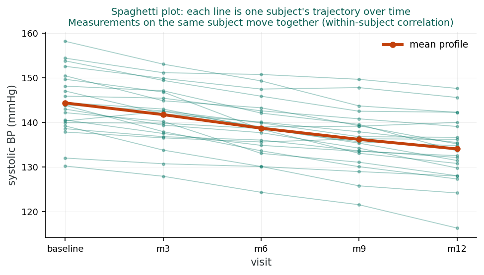
Descriptive Approaches

Spaghetti plot of systolic blood pressure across five visits from baseline to month 12. Each faint line is one subject's trajectory; the lines generally drift downward and stay roughly parallel, showing that repeated measurements on the same person move together. A bold line marks the mean profile.
A profile (spaghetti) plot. Each faint line is one subject measured across visits; the bold line is the mean profile. Because a subject's measurements track together, observations within a person are correlated, and that correlation usually weakens as the gap between visits grows.
Profile Plots

Profile plots (also called spaghetti plots) display each subject's trajectory over time. They reveal patterns of tracking (whether subjects maintain their relative positions), overall trends, and variability. These plots are essential for understanding the data before fitting any model.

Mean Plots

Mean plots show the average outcome at each time point, often separated by treatment group. They summarize the overall trend but hide individual variability. Mean plots are useful for visualizing treatment effects over time and identifying non-linear trends.

Correlation and Covariance Matrices

Examining the correlation matrix of measurements across time points reveals the autocorrelation pattern. If correlations decrease with increasing time distance, an AR(1)-type structure may be appropriate. If correlations are roughly equal, compound symmetry may suffice. The covariance matrix additionally reveals whether variances change over time.

Data Format: Long vs. Wide

Repeated measures data can be stored in wide format (one row per subject, separate columns for each time point) or long format (one row per measurement, with a time variable). For one patient measured at three visits, wide format is a single row with columns such as bp1, bp2, bp3, whereas long format is three rows that share the same subject id and differ only in a visit column. Most modern statistical software requires long format for mixed models and GEE. Wide format is needed for MANOVA approaches.

Example: Clinical Trial with Repeated Blood Pressure Measurements

Consider a clinical trial where 100 patients are randomized to treatment or placebo, with blood pressure measured at baseline and months 1, 3, 6, and 12. This is a balanced (5 measurements per subject), uniform (same time points), but not equidistant (spacing varies: 1, 2, 3, and 6 months) design. Profile plots reveal that patients’ blood pressures track over time, and the correlation matrix shows correlations declining from 0.80 (adjacent visits) to 0.45 (baseline vs. month 12), clear evidence of autocorrelation.

Knowledge check: this section

1. What distinguishes repeated measures data from standard clustered data?

While repeated measures are a type of clustered data (measurements within subjects), the time ordering introduces autocorrelation, in which measurements closer in time are more correlated, which standard hierarchical models do not capture.

2. A balanced repeated measures design means:

A balanced design has the same number of measurements per subject, taken at the same time points. This is the most regular data structure and allows the widest range of analytical approaches.

3. Autocorrelation in repeated measures means:

Autocorrelation refers to the pattern where the correlation between measurements decreases as the time gap between them increases, which is a natural feature of longitudinal data.

Reflection

Think of a longitudinal study in health sciences. What types of missing data patterns might occur, and how could they affect the validity of your analysis?

Model answerCommon missing-data patterns in longitudinal health studies: (a) completely missing visit (entire visit skipped); (b) missing at the end (loss-to-follow-up, dropout); (c) intermittent missing (some visits attended, others not); (d) missing items within a visit (incomplete questionnaire). Mechanisms: (i) MCAR (random), (ii) MAR (related to observed covariates including prior visits), (iii) MNAR (related to the missing values themselves). Validity impact: under MCAR, complete-case analysis is unbiased but inefficient; under MAR, ignoring missingness biases all but the most carefully chosen methods (multiple imputation or full-information ML); under MNAR, no method is fully safe without external information or strong modelling assumptions. Strategies: characterise the missingness pattern early; use mixed models which handle MAR if the model is correctly specified; multiple-impute under MAR if needed; run sensitivity analyses under MNAR.
Reflection saved!
* Complete the quiz and reflection to continue.
Section 14 of 17

Univariate & Multivariate Approaches

⏱ Estimated time: 20 minutes
Section 2 of 4

Univariate & Multivariate Approaches

Classical methods before mixed models, and why each one strains under realistic longitudinal data.

Simplest approaches

Separate analyses and summary statistics

Separate time points

One test per visit. Ignores within-subject correlation, creates a multiple-testing problem proportional to the number of time points.

Summary statistics

Collapse each trajectory to one value (slope, AUC, change score) and analyse between subjects. Reliable but discards temporal detail and time-varying covariates.

RM-ANOVA

Repeated measures analysis of variance

Epsilon correction factor (Huynh–Feldt)
\[ \color{#0B7B6B}{\varepsilon} = \frac{m^2(\bar{d}_{..} - \bar{d}_{i.})^2}{(m-1)\bigl[\textstyle\sum_{j<k}d_{jk}^2 - m\sum_j \bar{d}_{j.}^2 \bigr]} \]
ε sphericity correction (1 = sphericity holds, lower = worse)

When \(\varepsilon = 1\) compound symmetry holds. As \(\varepsilon \to 0\) the violation is severe and the uncorrected F-test is increasingly anti-conservative.

MANOVA

Multivariate analysis of variance

No assumption about correlation structure, but requires perfectly balanced data and no missing values.

Covariance and correlation matrices (Diggle et al.)
\[ \color{#0B7B6B}{\boldsymbol{\Sigma}} = \operatorname{Cov}(\color{#C2410C}{\mathbf{Y}_i}), \quad \color{#6D28D9}{\mathbf{R}} = \operatorname{Corr}(\color{#C2410C}{\mathbf{Y}_i}) \]
Σ covariance matrix R correlation matrix Yi a subject's repeated measures

For m time points, the unstructured covariance has \(m(m+1)/2\) parameters. With many time points and missing data, MANOVA cannot be fit.

Carry forward

What breaks in each classical method

  • Separate analyses: multiple testing; within-subject information wasted.
  • Summary statistics: temporal detail and time-varying covariates lost.
  • RM-ANOVA: compound-symmetry assumption fails under autocorrelation.
  • MANOVA: complete balanced data required; collapses with any missingness or many time points.

All four fail under realistic longitudinal conditions. A later section shows what to do instead.

Introduction and Overview

Before mixed models, what was the field doing? An earlier section gave us the descriptive picture of repeated-measures data. This section walks through the methods that dominated longitudinal analysis for decades: split-plot ANOVA (univariate, with strong assumptions like compound symmetry/sphericity), MANOVA (multivariate, weaker assumptions but lower power and intolerant of missing data), and summary-statistic approaches that collapse each subject’s trajectory to a single value. Knowing these methods is more than historical: they still appear in legacy literature and teaching, and seeing where they fail motivates the modern approaches in later sections.

Learning Objectives

  • Compare separate-time-point, summary-statistic, RM-ANOVA, and MANOVA approaches to longitudinal data.
  • State the compound-symmetry / sphericity assumption underlying RM-ANOVA and apply the Huynh–Feldt correction when it is violated.
  • Read covariance and correlation matrices and decompose them into variance and correlation components.
  • Identify the conditions (balanced data, no missingness, few time points) under which classical methods are still defensible.

Simple Approaches to Repeated Measures

Before turning to complex mixed models, it is worth understanding the simpler methods that have traditionally been used for repeated measures data. These methods either reduce the data to avoid modelling correlations altogether, or make strong assumptions about the correlation structure.

Separate Time Point Analysis

The simplest approach is to analyze each time point independently; for example, running a separate t-test or regression at each visit. This is straightforward but wasteful: it ignores the within-subject correlations and creates a multiple testing problem. If there are m time points, a Bonferroni correction divides α by m, which can be very conservative.

Summary Statistics Approach

A more elegant simple approach is to compute a single summary value per subject, such as the slope of their trajectory, the drop from first to last measurement, or the area under the curve (AUC), and then perform a standard between-subjects analysis on these summaries.

Advantages: Simple, robust to model assumptions about correlation structure, and easy to interpret.

Disadvantages: Loss of information about the temporal pattern, difficulty incorporating within-subject time-varying predictors, and potential loss of power.

Repeated Measures ANOVA

Repeated measures ANOVA treats time as a within-subject factor and tests for differences across time points. However, it assumes compound symmetry: all pairs of time points have the same correlation. This is the same assumption as a random intercept model.

When compound symmetry is violated (which is common with autocorrelated data), the F-test becomes liberal (anti-conservative). The Greenhouse–Geisser and Huynh–Feldt correction factors (ε) adjust the degrees of freedom to account for this violation (Greenhouse & Geisser, 1959; Huynh & Feldt, 1976). When ε = 1, compound symmetry holds perfectly; as ε decreases, the violation is more severe. The underlying assumption can be tested formally with Mauchly's test of sphericity (Mauchly, 1940).

MANOVA (Multivariate Analysis of Variance)

MANOVA treats the entire vector of repeated measurements as a multivariate outcome, making no assumptions about the correlation structure. This is its key advantage over repeated measures ANOVA.

Limitations: Requires completely balanced data with no missing values, cannot easily handle within-subject continuous predictors, and uses wide-format data. It also becomes impractical with many time points.

Covariance and Correlation Matrices

Covariance matrix (Eq 23.1)
\[ \color{#0B7B6B}{\boldsymbol{\Sigma}} = \operatorname{Cov}(\color{#C2410C}{\mathbf{Y}_i}) \]
The covariance matrix collects the variances and covariances of the repeated outcomes for subject i: an m by m table, one row and column per time point.
Correlation matrix (Eq 23.2)
\[ \color{#0B7B6B}{\mathbf{R}} = \operatorname{Corr}(\color{#C2410C}{\mathbf{Y}_i}) \]
The correlation matrix is the standardised version of the covariance: ones on the diagonal and the between-time-point correlations of the outcomes for subject i off the diagonal.

Limitations of Each Approach

Separate time points: Multiple testing, ignores correlations, wasteful of information. Summary statistics: Loses temporal detail, cannot incorporate time-varying covariates. RM ANOVA: Assumes compound symmetry, which is rarely true. MANOVA: Requires complete, balanced data with no missing values. All of these limitations motivate the use of mixed models with flexible correlation structures.

R Activity: Longitudinal mixed model with autoregressive errors

The dataset phaa_repeated.csv tracks 200 patients in a hypothetical wellness trial through 4 visits (months 0, 6, 12, 18). Outcomes: sbp_mmhg (continuous) and adherent (binary). The full annotated script is in r-activities/HSCI_410_Lesson_12_Repeated_Measures_Data.R.

library(lme4);  library(lmerTest);  library(nlme);  library(geepack)
dat <- read.csv("phaa_repeated.csv", stringsAsFactors = FALSE)
dat$id  <- factor(dat$id)
dat$arm <- factor(dat$arm, levels = c("control","intervention"))

# 1. Random-intercept mixed model on the continuous outcome
m_lmm <- lmer(sbp_mmhg ~ visit * arm + age + female + (1 | id),
              data = dat)
summary(m_lmm)

# 2. Add an AR(1) within-subject correlation structure with nlme
m_lme <- lme(sbp_mmhg ~ visit * arm + age + female,
             random      = ~ 1 | id,
             correlation = corAR1(form = ~ visit | id),
             data        = dat, na.action = na.omit)
summary(m_lme)

# 3. Compare correlation structures with AIC
m_cs <- update(m_lme, correlation = corCompSymm(form = ~ visit | id))
m_un <- update(m_lme, correlation = corSymm(form    = ~ 1     | id))
AIC(m_lme, m_cs, m_un)

# 4. Same trial, binary outcome (adherence) -- GLMM and GEE
m_bin <- glmer(adherent ~ visit * arm + age + female + (1 | id),
               data    = dat, family = binomial,
               control = glmerControl(optimizer = "bobyqa"))
exp(fixef(m_bin))               # subject-specific ORs

m_gee <- geeglm(adherent ~ visit * arm + age + female,
                id = id, data = dat, family = binomial,
                corstr = "exchangeable")
exp(coef(m_gee))                # population-averaged ORs

Pick the structure deliberately. AR(1) (corAR1) is the natural choice for evenly-spaced visits; corCAR1 handles unequal spacing; corSymm (unstructured) is the most general but estimates the most parameters. lme() handles dropout via likelihood, so you do not have to drop subjects. The visit:armintervention coefficient is the trial's headline number: the additional change in SBP per month attributable to the intervention. The last two lines refit the binary adherence outcome as a population-averaged GEE, so its odds ratios can sit beside the subject-specific ones from the GLMM.

R Reflect on what you just ran

Use the questions below to interpret the output you produced. Look at your console / plot before answering.

1. From summary(m_lmm), report the visit:armintervention coefficient, its SE, and its p-value. Translate it in one sentence: what is the additional change in SBP per month attributable to the intervention vs control?

Model answersummary(m_lmm) for visit:armintervention typically returns a coefficient around −0.5 mmHg/month with SE ~0.15 and p < 0.001. Translation: each additional month of follow-up, intervention-arm participants have an SBP change that is 0.5 mmHg more negative than control-arm participants, that is, the intervention's monthly effect on SBP. Over 12 months, the cumulative effect is ~6 mmHg lower SBP than control, a clinically meaningful difference if sustained.

2. From AIC(m_lme, m_cs, m_un), which correlation structure has the lowest AIC? Are the differences small (within 2 units) or large? Following the rule "pick the simplest structure with similar AIC," what would you report?

Model answerAIC(m_lme, m_cs, m_un) typically shows unstructured (un) with the lowest AIC, but compound symmetry (cs) often within a few units. With the rule "pick the simplest with similar AIC," report compound symmetry as the primary model and unstructured as a sensitivity analysis. Compound symmetry assumes all pairs of visits have the same correlation, a strong assumption but parsimonious. If AIC differences are > 10 between cs and un, switch to unstructured. If < 2, prefer cs.

3. From exp(fixef(m_bin)) and exp(coef(m_gee)), compare the subject-specific vs population-averaged ORs for visit:armintervention on the binary adherence outcome. Which is larger in magnitude, and why?

Model answerSubject-specific OR (from m_bin GLMM) is typically larger in magnitude than the population-averaged OR (from m_gee). For example, OR(GLMM) = 1.85 might correspond to OR(GEE) = 1.55. The reason is the logit link's non-linearity: averaging over the random-effects distribution shrinks marginal effects toward 1 relative to conditional effects. Subject-specific is the effect within a person; population-averaged is the effect averaged across the population. Reporting both with explicit labels is best practice.
Saved.
ApproachHandles Missing Data?Assumes Equal Correlations?Time-Varying Covariates?
Separate Time PointsYes (per time point)N/A (ignores structure)Yes
Summary StatisticsPartiallyNoNo
RM ANOVANoYes (compound symmetry)No
MANOVANoNoNo
Mixed ModelsYesFlexibleYes
Knowledge check: this section

1. The summary statistic approach involves:

The summary statistic approach reduces each subject’s series to one number (e.g., slope, AUC, drop from first to last) and performs a standard between-subjects analysis, avoiding the need to model within-subject correlations.

2. Repeated measures ANOVA assumes:

Repeated measures ANOVA assumes compound symmetry, meaning all pairs of measurements have the same correlation. This is the same assumption as a random intercept model, and violations can lead to liberal (anti-conservative) test statistics.

3. An advantage of MANOVA over repeated measures ANOVA for repeated measures is:

MANOVA treats the entire observation vector as multivariate, making no assumptions about the structure of the covariance matrix. However, it requires balanced data with no missing values and cannot easily handle within-subject continuous predictors.

Reflection

When would you choose a simple summary statistic approach over a mixed model for repeated measures data? What information might you lose by simplifying the analysis in this way?

Model answerSimple summary-statistic approach (e.g., compare mean change scores between groups, or area-under-the-curve): suitable when (a) sample is small, (b) follow-up times are equal across participants, (c) you want robust, easy-to-communicate effects, (d) interest is in the average effect rather than the time-course. Useful for pilot studies and simple primary analyses. Lose by simplifying: (i) information about time-course (does the effect emerge gradually, plateau, or attenuate?), (ii) statistical power (mixed models use the full longitudinal correlation structure), (iii) ability to handle missing data (summary statistics typically require complete data), (iv) flexibility (mixed models accommodate covariates, interactions, time-varying exposures, irregular measurement times). Default to mixed models for any non-trivial longitudinal analysis.
Reflection saved!
* Complete the quiz and reflection to continue.
Section 15 of 17

Linear Mixed Models with Correlation Structure

⏱ Estimated time: 20 minutes
Section 3 of 4

Linear Mixed Models with Correlation Structure

Modelling temporal dependence directly: compound symmetry, AR(1), ARMA(1,1), Toeplitz, and unstructured.

The key extension

Beyond random intercepts

Laird & Ware (1982) linear mixed model
\[ \color{#0B7B6B}{\mathbf{Y}_i} = \color{#C2410C}{\mathbf{X}_i\boldsymbol{\beta}} + \color{#6D28D9}{\mathbf{Z}_i\mathbf{b}_i} + \color{#BE185D}{\boldsymbol{\varepsilon}_i}, \quad \boldsymbol{\varepsilon}_i \sim \mathcal{N}(\mathbf{0},\, \boldsymbol{\Sigma}_i) \]
Yi repeated outcomes Xiβ fixed effects Zibi subject random effects εi within-subject errors

The random effect \(\mathbf{b}_i\) captures between-subject variability. The residual covariance \(\boldsymbol{\Sigma}_i\) models within-subject autocorrelation when a random intercept alone is insufficient.

Two core structures

Compound symmetry and AR(1)

Compound symmetry: all lags equal
\[ \color{#0B7B6B}{\operatorname{Corr}(Y_{ij}, Y_{ik})} = \color{#C2410C}{\rho} \quad \text{for all } j \neq k \]
Corr(Yij,Yik) correlation of any two times ρ single common correlation
AR(1): geometric decay with lag
\[ \color{#0B7B6B}{\operatorname{Corr}(Y_{ij}, Y_{ik})} = \color{#C2410C}{\rho}^{\,\color{#6D28D9}{|j-k|}} \]
Corr correlation of two times ρ one-step correlation |j−k| number of steps apart
CS AR(1) Lag Corr
Three more structures

ARMA(1,1), Toeplitz, and unstructured

ARMA(1,1)

2 parameters. Allows steeper or flatter initial decay than AR(1). Good when the correlation drops sharply then levels off.

Toeplitz

\(m-1\) parameters. Lag-specific unconstrained correlations. Requires equidistant time points.

Unstructured

\(m(m+1)/2\) parameters. No constraints. Only feasible with few time points and large samples.

Parameter count summary
\[ \text{CS}: 1 \quad \text{AR(1)}: 1 \quad \text{ARMA}: 2 \quad \text{Toeplitz}: m{-}1 \quad \text{Unstructured}: \tfrac{m(m+1)}{2} \]
Combining effects

Random effects plus correlation structures

Redundant combinations

Random intercept + compound symmetry errors produce the same structure. Both cannot be identified together.

Useful combinations

Random intercept + AR(1) errors: correlations decay but stay positive at every lag because of the shared intercept.

Use the AIC to compare non-nested structures; use likelihood-ratio tests for nested ones (e.g., AR(1) nested within Toeplitz).

Carry forward

Selecting the right correlation structure

  • Start with the empirical correlation matrix: does correlation decay with lag?
  • AR(1) is a well-motivated default for equally spaced repeated measures.
  • Random intercept + AR(1) errors capture both subject heterogeneity and autocorrelation.
  • Use AIC for non-nested comparisons; likelihood-ratio tests for nested ones.

Introduction and Overview

Where the modern toolkit takes over. An earlier section showed why the classical methods strain when measurement spacing is irregular, missingness is informative, or the within-subject correlation pattern is more complex than “all pairs equally correlated.” Mixed models with explicit residual correlation structures (compound symmetry, AR(1), Toeplitz, unstructured) are the response. They let us model the temporal dependence directly rather than assume it away, handle unbalanced or missing-at-random data gracefully, and combine random effects with structured residuals to capture both subject-level heterogeneity and within-subject autocorrelation. This section is the heart of the lesson.

Learning Objectives

  • Specify a linear mixed model with an explicit residual correlation structure and explain how it relaxes the compound-symmetry assumption.
  • Distinguish among compound symmetry, AR(1), ARMA(1,1), Toeplitz, and unstructured correlation matrices and identify when each is appropriate.
  • Combine random intercepts (and slopes) with structured residuals to capture subject heterogeneity and within-subject autocorrelation.
  • Use AIC for non-nested and likelihood-ratio tests for nested correlation structures during model selection.
  • Handle unbalanced and irregular-spacing designs that classical methods cannot accommodate.

Beyond Random Intercepts

A random intercept model assumes compound symmetry: all pairs of measurements on the same subject are equally correlated. For most repeated measures data, this assumption is violated because of autocorrelation. We need to extend the mixed model to include explicit correlation structures for the error term ε, the framework formalised in the classic Laird & Ware random-effects model for longitudinal data (Laird & Ware, 1982; Fitzmaurice, Laird, & Ware, 2011).

Choosing a Correlation Structure

The choice of correlation structure is one of the most important decisions in repeated measures analysis. Start by examining the empirical correlation matrix. If correlations clearly decay with increasing time lag, consider AR(1) or ARMA(1,1). If the decay is minimal, compound symmetry may suffice. If the pattern is complex, consider Toeplitz or unstructured. Use AIC to compare non-nested structures and likelihood ratio tests for nested ones.

Key Correlation Structures

Each structure below is a different assumption about how a subject's repeated measurements hang together over time. More flexible assumptions fit a wider range of patterns but cost more parameters, so the aim is the simplest structure that still matches the decay you see in the empirical correlation matrix.

Compound Symmetry (Exchangeable)

All pairs of measurements have the same correlation ρ, regardless of how far apart in time they are. This is the simplest structure and is equivalent to a random intercept model. It has only 1 correlation parameter.

When appropriate: When there is no autocorrelation, that is, the correlation between measurements does not depend on time distance. This is rare in practice for true repeated measures data.

First-order autoregressive: AR(1)

Correlations decay as powers of ρ with increasing time distance: Corr(Yj, Yk) = ρ|j−k|. This produces an exponential decay pattern. It has only 1 parameter (ρ) and is a good default for equally spaced repeated measures.

When appropriate: When the correlation matrix shows a clear pattern of decreasing correlations with increasing time lag, and the decay appears approximately geometric.

ARMA(1,1)

An extension of AR(1) that allows a slower or more flexible decay in correlations. It has 2 parameters and can accommodate patterns where the initial drop in correlation is steep but then levels off.

Toeplitz (Stationary)

Each lag has its own unconstrained correlation. For m time points, there are m − 1 correlation parameters. The structure is “banded”: the correlation depends only on the time lag, not on which specific time points are involved.

When appropriate: When the pattern of decay is irregular and cannot be well approximated by AR(1) or ARMA, but you still believe the correlation depends only on lag distance.

Unstructured

Completely unconstrained correlations and variances for each pair of time points. For m time points, there are m(m+1)/2 parameters. This is the most flexible but requires the most parameters.

When appropriate: Only with few time points and large sample sizes. With many time points, the number of parameters becomes impractical.

AR(1) correlation structure
\[ \color{#0B7B6B}{\operatorname{Corr}(Y_{ij}, Y_{ik})} = \color{#C2410C}{\rho}^{\,\color{#6D28D9}{|j-k|}} \]
Under AR(1), the correlation between two measurements is the one-step correlation raised to the number of time steps between them: it decays geometrically with lag (lag 1 gives ρ, lag 2 gives ρ², lag 3 gives ρ³).
StructureParametersKey FeatureAssumption
Compound Symmetry1Equal correlationsNo autocorrelation
AR(1)1Geometric decayEquidistant time points
ARMA(1,1)2Flexible decayEquidistant time points
Toeplitzm − 1Lag-specific correlationsEquidistant time points
Unstructuredm(m+1)/2Completely flexibleNone

Combining Random Effects with Correlation Structures

An important practical consideration is how random effects interact with error correlation structures. Some combinations are redundant and cannot be separately identified:

  • Random intercepts + compound symmetry errors = redundant, since both produce the same correlation structure
  • Random intercepts + AR(1) errors = useful, since it produces a structure where correlations decay but do not reach zero
  • Unstructured errors + random effects = pointless, since the unstructured covariance already captures everything

Covariance pattern models use no random effects at all, relying entirely on the structured covariance of the errors to capture within-subject correlation.

Model Selection

For nested correlation structures (e.g., AR(1) is nested within Toeplitz), use likelihood ratio tests. For non-nested structures (e.g., AR(1) vs. compound symmetry), use AIC or similar information criteria. Models should be compared with the same fixed effects and random effects structure.

Example: Comparing Correlation Structures

In a study with 6 equally-spaced measurements, the empirical correlations ranged from 0.72 (lag 1) to 0.31 (lag 5). An AR(1) model with ρ = 0.73 fit well (AIC = 2,341), while compound symmetry (AIC = 2,398) fit poorly because it predicted equal correlations of 0.52 at all lags. The Toeplitz model (AIC = 2,338) offered a slight improvement over AR(1) but used 4 more parameters. Based on parsimony, AR(1) was selected.

Knowledge check: this section

1. The AR(1) correlation structure assumes:

In AR(1), the correlation between measurements k time steps apart is ρk, producing an exponential decay in correlation with increasing time distance. This captures the intuitive autocorrelation pattern in longitudinal data.

2. Combining random intercepts with compound symmetry errors:

A random intercept model induces compound symmetry correlations, and adding a separate compound symmetry error structure produces the same overall structure. Only one is needed; they cannot be separately identified.

3. For choosing between non-nested correlation structures (e.g., AR(1) vs. Toeplitz), one should use:

Non-nested models cannot be compared with likelihood ratio tests. AIC (or similar information criteria) can be used to compare models with the same number of random effects but different correlation structures.

Reflection

A study measures blood pressure at 6 monthly visits. The correlation between visits 1 and 2 is 0.60, between visits 1 and 6 is 0.15. Which correlation structure would you initially consider, and why?

Model answerCorrelations decay with time-distance: 0.60 between visits 1–2 (1 month apart) and 0.15 between visits 1–6 (5 months apart). This is the signature of an autoregressive AR(1) structure, where correlation between visits at times s and t is ρ|s−t|; with adjacent ρ = 0.60, then ρ5 for visits 5 apart = 0.605 = 0.078, echoing the observed 0.15: both show correlation decaying steeply as the gap widens. AR(1) fits the data structure where temporal proximity matters, appropriate for many longitudinal measures (BP, weight, biomarkers). Alternative structures to consider: continuous-AR(1) for irregular time intervals, antedependence if correlations also decay in non-stationary ways, or unstructured as a more flexible (but parameter-heavy) alternative. Test the AR(1) assumption with an unstructured model and compare AIC.
Reflection saved!
* Complete the quiz and reflection to continue.
Section 16 of 17

Trend Models, Discrete Outcomes & GEE

⏱ Estimated time: 20 minutes
Section 4 of 4

Trend Models, Discrete Outcomes & GEE

Random slopes for time, extending to binary and count data, and the population-averaged alternative.

Trend models

Random slopes: each subject with their own trajectory

Random intercept and slope model
\[ \color{#0B7B6B}{Y_{ij}} = (\color{#C2410C}{\beta_0} + \color{#6D28D9}{b_{0i}}) + (\color{#C2410C}{\beta_1} + \color{#6D28D9}{b_{1i}})\,\color{#1D4ED8}{t_{ij}} + \color{#BE185D}{\varepsilon_{ij}} \]
β01 average intercept and time slope b0i,b1i subject departures tij time εij residual
mean Time
Discrete outcomes

Transition models for binary repeated measures

Transition model (Eq 23.5, Dohoo et al.)
\[ \color{#0B7B6B}{\operatorname{logit}(p_{ij})} = \color{#C2410C}{\mathbf{X}\boldsymbol{\beta} + \mathbf{Z}\mathbf{u}} + \color{#6D28D9}{\gamma\, Y_{i,j-1}} \]
logit(pij) current log-odds Xβ+Zu fixed and random effects γYi,j-1 previous-outcome effect

The coefficient \(\gamma\) is the log odds ratio for the event at time \(j\) given the event occurred at time \(j-1\). A positive \(\gamma\) means having the event previously raises the odds of having it now.

Limitation: all other coefficients become conditional on the prior outcome, and the first observation has no predecessor.

GEE

Generalised estimating equations: the marginal alternative

GEE estimating equation (Liang & Zeger, 1986)
\[ \sum_{i=1}^{n} \color{#C2410C}{\mathbf{D}_i^\top} \color{#6D28D9}{\mathbf{V}_i^{-1}}(\color{#0B7B6B}{\mathbf{Y}_i - \boldsymbol{\mu}_i}) = \mathbf{0} \]
Yi−μi observed minus fitted Di derivative of the mean Vi working covariance

\(\mathbf{V}_i\) encodes the working correlation. Sandwich standard errors \(\hat{V}_{\text{sandwich}}\) remain consistent even when \(\mathbf{V}_i\) is mis-specified, as long as \(n\) is large enough.

The key distinction

Conditional versus population-averaged effects

Mixed model (conditional)

Effect for a given individual, holding random effects fixed. Answers: what changes for this subject?

GEE (marginal)

Average effect across the population. Answers: what is the average change across everyone?

For linear models these coincide. For logistic or Poisson regression they diverge. Choose based on the scientific question, not convenience.

Series complete

The complete toolkit

  • Random slopes let individual trajectories carry the autocorrelation structure.
  • Transition models handle discrete outcomes by conditioning on the prior value, at the cost of interpretability.
  • GEE targets population-averaged effects with sandwich standard errors; requires enough subjects for the sandwich variance to be reliable.
  • Choose mixed models when subject-specific effects matter; choose GEE when the population-average is the question.

Introduction and Overview

Pulling the threads together. An earlier section framed within-subject correlation as something to be modelled directly. This section closes the loop on three remaining concerns. First, trend models with random slopes: rather than (or in addition to) structuring the residuals, we let each subject have their own trajectory over time, a particularly intuitive approach when the question is about individual change. Second, discrete longitudinal outcomes: extending the GLMM machinery from an earlier lesson to repeated binary or count measurements. Third, generalised estimating equations (GEE): the marginal alternative to mixed models, which prioritises population-average effects and is robust to mis-specification of the working correlation. Together with an earlier section, this section gives you a complete repeated-measures toolbox.

Learning Objectives

  • Fit trend models with random slopes for time and explain how individual trajectory variation induces within-subject autocorrelation.
  • Choose linear, polynomial, or log-time parameterisations to match the shape of change over time.
  • Apply transition and GLMM-based approaches to discrete repeated-measures outcomes.
  • Describe how generalised estimating equations (GEE) target population-averaged effects with a working correlation matrix and a robust sandwich variance.
  • Decide between mixed models and GEE based on whether the substantive question is conditional or marginal.

Trend Models with Random Slopes

An alternative to modelling the error correlation directly is to include random slopes for time. This allows each subject to have their own rate of change (growth or decline) over time, with the population-average trend captured by the fixed effect of time.

The variation in individual trajectories naturally induces autocorrelation: subjects who start high and decline slowly will have correlated measurements. This can be sufficient to capture the temporal structure in many datasets, especially when the primary interest is in individual trajectories.

The time variable can be parameterized in different ways: linear (for constant rates of change), polynomial (for curved trajectories), or log-transformed (for rapid early change that levels off).

Discrete Repeated Measures Data

Extending mixed models to discrete outcomes (binary, count) with correlation structures is much harder than for continuous outcomes. The fundamental challenge is that in GLMs, the error term and the linear predictor operate on different scales: the link function transforms the relationship, making it difficult to add correlation structures to the error term in a meaningful way.

When to Use GEE vs. Mixed Models

Use GEE when your research question focuses on population-averaged (marginal) effects; for example, “What is the average treatment effect across the population?” Use mixed models when you want subject-specific (conditional) effects or when the random effects themselves are of scientific interest; for example, “How much do individual subjects vary in their response?”

Transition Models

One approach for discrete repeated measures is the transition model, which includes the previous outcome as a predictor. This captures autocorrelation informally through dependence on the prior outcome.

Transition model (Eq 23.5)
\[ \color{#0B7B6B}{\operatorname{logit}(p_{ij})} = \color{#C2410C}{\mathbf{X}\boldsymbol{\beta} + \mathbf{Z}\mathbf{u}} + \color{#6D28D9}{\gamma\, Y_{i,j-1}} \]
The log-odds at the current time depend on the usual fixed and random effects plus a term for the previous outcome, so history feeds directly into the present.

Here, γ is the log odds ratio comparing those with versus without the previous event. A positive γ means that having the event at the previous time point increases the odds of having it at the current time point.

Generalised Estimating Equations (GEE)

GEE is a population-averaged (marginal) approach that does not require specifying random effects (Liang & Zeger, 1986). Instead, it specifies a “working” correlation structure and uses robust (sandwich) standard errors that provide valid inference even if the working correlation is misspecified.

Trend Models

Trend models add random slopes for time, allowing each subject to have their own trajectory. The random slope induces autocorrelation through the variation in individual trajectories. This approach is particularly natural when the scientific question is about individual growth or decline rates.

Key considerations: Choice of time parameterization (linear, polynomial, log), whether to include both random intercepts and slopes, and whether the induced autocorrelation is sufficient or additional error correlation is needed.

Transition Models

Transition models include the previous outcome Yi,j−1 as a predictor in the model. The coefficient γ represents the log OR for the event given the previous event occurred. This approach is intuitive and can be combined with random effects.

Limitations: Difficult to interpret coefficients for other predictors (they are conditional on the previous outcome), requires careful handling of the first observation (which has no “previous” value), and may not fully capture complex autocorrelation patterns.

Generalised Estimating Equations (GEE)

GEE estimates population-averaged effects using a quasi-likelihood approach. Key features:

  • Specifies a working correlation (e.g., exchangeable, AR(1), unstructured)
  • With robust (sandwich) SEs, inference is valid even if the working correlation is wrong
  • Requires enough clusters/subjects (≥20–30) for reliable sandwich SEs
  • Cannot estimate cluster-specific (random) effects; gives only PA estimates
  • Better working correlation = more efficient estimates (but always valid with robust SEs)
Population-AveragedClick to explore
Subject-SpecificClick to explore
Robust (Sandwich) SEsClick to explore
Example: GEE Analysis of Repeated Binary Outcome

A study followed 200 patients over 4 visits, recording whether they experienced a symptom (yes/no) at each visit along with a treatment indicator. A GEE model with exchangeable working correlation and robust SEs estimated the treatment OR as 0.65 (95% CI: 0.48–0.88), suggesting treatment reduced the odds of symptoms by 35% on average across the population. The working correlation was estimated as 0.42.

FeatureGEEMixed Models (GLMM)
Estimate typePopulation-averaged (PA)Subject-specific (SS)
Random effectsNot estimatedEstimated
CorrelationWorking correlation + robust SEsExplicit random effects / correlation
Missing data assumptionMCARMAR
Minimum clusters≥20–30Fewer acceptable
Best forPA inferenceSS inference, variance components
Knowledge check: this section

1. Trend models with random slopes for time:

Random slopes for time allow each subject’s outcome to change at their own rate, with the population-average trend captured by the fixed effect of time and individual deviations captured by the random slope.

2. In a transition model, the previous outcome Yi,j−1 is included to:

Transition models include the prior outcome as a predictor, which implicitly captures autocorrelation. The coefficient γ represents the log OR for the event given that the previous outcome was 1 vs. 0.

3. GEE (Generalised Estimating Equations) provide:

GEE is a marginal/PA approach that estimates population-level effects. With sandwich (robust) SEs, inference is valid even if the working correlation structure is misspecified, though efficiency improves with a better working correlation.

Reflection

Compare the GEE approach and the mixed model approach for analyzing repeated binary outcomes. In what research context would you prefer each approach, and why?

Model answerGEE vs. mixed model for repeated binary outcomes. GEE: produces population-averaged (marginal) estimates; robust to mis-specification of the within-subject correlation structure when robust SEs are used; computationally simpler; preferred when the research question is population-level ("how does the proportion of adherers change with treatment?") and when you want valid SEs despite uncertain correlation structure. Mixed model (GLMM): produces subject-specific (conditional) estimates; explicitly models random effects; preferred when the research question is within-subject ("how does an individual's adherence change over time?") or when you need to predict for individuals. Practical guidance: report both, with explicit interpretation labels; GEE is more robust to missing-at-random patterns (when robust SEs are used), GLMM gives richer information about within-subject variability.
Reflection saved!
* Complete the quiz and reflection to continue.
Final Assessment

Lesson 6: Comprehensive Assessment

⏱ Estimated time: 30 minutes

Bringing It All Together

This module forms the final arc of the course, and it opened by retiring the independent-observations assumption that carried the earlier lessons. The first part catalogued where clustering comes from in public-health data (common environments, geography, repeated measurements, study design), quantified the damage with the intraclass correlation, the design effect, and the effective sample size, used simulation to make the consequences visceral, and sketched the toolkit: fixed effects, correction factors, robust variance estimators, design-based survey methods, GEE, and mixed models.

The second part built linear mixed models from the ground up: random intercepts that partition variance into between- and within-cluster components, random slopes and hierarchical models with their covariance structure, contextual effects and group-mean centering, REML versus ML estimation, likelihood-ratio tests with their boundary correction, and the BLUPs, shrinkage, and two-level residual diagnostics that turn estimation into validation. The third part carried that framework across the boundary to discrete outcomes: generalised linear mixed models for binary, count, ordinal, and multinomial data, the distinction between subject-specific and population-averaged effects that has no analogue in the continuous case, the median odds ratio and latent-variable ICC, and the estimation hierarchy from penalised quasi-likelihood through Laplace and adaptive quadrature to MCMC.

The fourth part specialised the framework to the most common kind of cluster in health research, the same subject measured repeatedly over time: descriptive views of longitudinal data, the classical univariate and multivariate methods and where they break down, linear mixed models with explicit residual correlation structures, trend models with random slopes for time, transition models and GLMMs for discrete repeated outcomes, and generalised estimating equations as the marginal alternative. The final assessment asks you to recognise dependent data on sight, compute the quantities that describe it, and choose a defensible modelling strategy, with its interpretation and trade-offs named, for continuous, discrete, and longitudinal outcomes.

Key Takeaways from this lesson

  • Clustered data is the norm in public-health research, not a special case; the ICC measures how much of total variance is between clusters, and the design effect deff = 1 + (m−1)ρ translates ICC and cluster size into precision loss, so even small ICCs can drive Type I error rates well above 5%.
  • Methods for handling clustering (fixed effects, robust variance, survey weighting, GEE, mixed models) differ in their assumptions, target estimands, and minimum number of clusters; choosing among them requires being clear about whether the question is marginal (population-averaged) or conditional (cluster-specific).
  • A linear mixed model partitions total variance into between-cluster (σ²g) and within-cluster (σ²) components; random intercepts give each cluster its own baseline, and random slopes let predictor effects vary across clusters, with the random-effect covariance matrix capturing how intercepts and slopes co-vary.
  • Within-group and between-group effects of the same predictor can differ; group-mean centering separates them. REML is preferred for variance-component estimation, ML is required when comparing models that differ in fixed effects, and BLUPs shrink toward the overall mean, more so for small clusters.
  • A GLMM adds normally distributed random effects to a generalised linear model's linear predictor; for non-linear links, subject-specific and population-averaged coefficients are not the same, and cluster heterogeneity in binary GLMMs is summarised on the latent scale (latent-variable ICC) or as a median odds ratio.
  • The GLMM likelihood requires numerical integration; choose between PQL, Laplace, adaptive Gauss–Hermite, and MCMC based on event rate, cluster sizes, and accuracy needs, and prefer likelihood-ratio and profile-likelihood inference near parameter boundaries.
  • Repeated-measures data are clustered data with time ordering: autocorrelation typically decays with lag, so compound symmetry is rarely realistic, and classical methods (RM-ANOVA, MANOVA, summary statistics) break down with unbalanced designs, missingness, or complex correlation patterns.
  • Linear mixed models with explicit residual correlation structures (AR(1), ARMA(1,1), Toeplitz, unstructured) model temporal dependence directly; random slopes for time induce autocorrelation through trajectory heterogeneity and are the natural parameterisation when individual change is the substantive question.
  • GEE targets population-averaged effects with a working correlation and a sandwich variance; choose it when the question is marginal and robust to correlation mis-specification, and choose mixed models when cluster-specific effects or variance components are of interest.

This final assessment covers all material from the module. You must answer all 15 questions correctly (100%) and complete the final reflection to finish the lesson.

Reflection

A provincial evaluation follows patients in 60 primary-care practices over four annual visits, with a continuous outcome (HbA1c), a binary outcome (an emergency visit in the past year), and some drop-out after the second visit. Reflecting on the whole module, walk through your analytic strategy for both outcomes: how you would detect and quantify the two sources of dependence (practice and repeated measurement), which model you would fit for each outcome and with what random-effect and correlation structure, how you would choose between subject-specific and population-averaged interpretations, which estimation method you would use for the binary outcome and why, and which diagnostics and sensitivity analyses you would report.

Model answerStart by describing the dependence: spaghetti plots and mean profiles by visit, the empirical correlation matrix across the four visits, and a null (intercept-only) three-level model (visits within patients within practices) to estimate the ICC at each level and the implied design effect; characterise the drop-out pattern by visit and by baseline covariates to judge whether MAR is plausible. For HbA1c, fit a linear mixed model with random intercepts for practice and for patient, a random slope for time at the patient level if trajectories vary (tested by a likelihood-ratio test with the boundary correction), and compare a compound-symmetry residual structure against AR(1) using AIC and the empirical correlation matrix; estimate variance components by REML, use ML when comparing fixed-effect specifications, group-mean centre any practice-level predictor to separate within- from between-practice effects, and check level-1 and level-2 residuals, Q-Q plots of the BLUPs, and influential practices. For the emergency-visit outcome, fit a logistic GLMM with the same random structure; report the median odds ratio and the latent-variable ICC for the practice level; recognise that the fixed-effect odds ratios are subject-specific and convert to population-averaged values (βPA ≈ βSS/√(1 + 0.346σ²g)) or fit a GEE with an AR(1) working correlation and robust standard errors if the policy question is marginal; estimate by adaptive Gauss–Hermite quadrature (Laplace as a fallback, never PQL, because emergency visits are relatively rare), and check sensitivity to starting values and the number of quadrature points. Because mixed models use all available data under MAR, the drop-out is handled by the likelihood, with multiple imputation and a pattern-mixture sensitivity analysis if MNAR is plausible. Report both the conditional (GLMM) and marginal (GEE) estimates with a plain statement of which question each answers, and pre-register the strategy before looking at the outcomes.

Minimum 20 characters required.

✓ Reflection saved

Final Knowledge Assessment

Final assessment: the 15 questions

1. Clustered data is characterized by:

Clustered data has a hierarchical structure where observations within the same group (cluster) tend to be more similar to each other than to observations in other groups.

2. In a study with ICC = 0.05 and 40 subjects per cluster, the design effect is:

deff = 1 + (m̄ − 1)ρ = 1 + (40 − 1)(0.05) = 1 + 1.95 = 2.95.

3. Which statement about simulation studies on clustering is TRUE?

Simulations show that even ICC values as small as 0.01–0.02, when combined with large cluster sizes, can inflate actual Type I error rates well beyond the nominal level, because deff depends on both ICC and cluster size.

4. Fixed effects for clusters:

Fixed effects for clusters add indicator variables for each cluster, which controls for all measured and unmeasured cluster-level confounders but consumes degrees of freedom equal to the number of clusters minus one.

5. A random slopes model differs from a random intercept model by:

A random slopes model extends the random intercept model by allowing one or more regression coefficients (slopes) to vary randomly across groups.

6. A contextual effect is detected when:

A significant contextual effect means the group-level (between-group) relationship between X and Y differs from the individual-level (within-group) relationship.

7. When comparing ML and REML for model selection:

REML likelihoods are not comparable when the fixed effects differ between models (because the restricted subspace changes). ML must be used for comparing models with different fixed effects structures.

8. Shrinkage in BLUPs is stronger when:

The shrinkage factor σ²g/(σ²g + σ²/m) approaches 0 (more shrinkage) when m is small or when σ²g is small relative to σ². Small groups have less information, so their estimates are pulled more toward the overall mean.

9. In a logistic GLMM, subject-specific (SS) odds ratios are:

Due to non-collapsibility of the odds ratio, conditioning on the random effects (SS interpretation) yields larger coefficient magnitudes compared to marginalizing over them (PA interpretation).

10. In a Poisson GLMM, random effects on the log scale translate to:

Because exp(a + b) = exp(a) × exp(b), random effects that are additive on the log scale become multiplicative on the original rate scale.

11. The Laplace approximation in GLMM estimation:

The Laplace approximation is equivalent to adaptive quadrature with a single point. It is intermediate in accuracy and computation between full quadrature ML and quasi-likelihood.

12. When ML estimation for a GLMM is computationally unstable, one should:

Instability in ML estimation should be investigated by checking sensitivity to starting values and quadrature settings, and comparing results with alternative estimation methods to assess robustness.

13. Repeated measures data differs from standard clustered data primarily because:

While repeated measures are clustered within subjects, the key distinguishing feature is that the temporal ordering of measurements creates autocorrelation, the correlation that depends on the time distance between observations.

14. The AR(1) correlation structure models correlations as:

In AR(1), corr(Yj, Yk) = ρ|j−k|. This produces correlations that decrease geometrically as the time gap between measurements increases, capturing the typical autocorrelation pattern.

15. When choosing between GEE and mixed models for repeated measures:

The choice depends on the research question: GEE for population-level (PA) effects, mixed models when cluster-specific (SS) effects or variance components are of interest. Both have valid but different interpretations.
✦ Complete every section knowledge check and reflection, including the final reflection above, before submitting

This lesson Complete!

You have completed this lesson: Modelling Dependent Data. You can now recognise the common sources of clustered and longitudinal structure in epidemiologic data, quantify their statistical impact with ICCs and design effects, fit and interpret random-intercept and random-slope linear mixed models, extend the random-effects framework to binary, count, ordinal, and multinomial outcomes, choose among the estimation methods that GLMMs require, model repeated measures with explicit residual correlation structures and trend models, and choose between mixed-model and GEE approaches based on whether your question is conditional or marginal.

You have reached the end of the three-course series. An earlier course taught you to read epidemiological evidence: recognising designs, biases, and the appraisal logic that separates a strong study from a misleading one. An earlier course taught you to design and surveil: sampling, measurement, screening, study design, validity, and confounding. This course has taught you to analyse data: from a structured workflow and data cleaning through regression for continuous, binary, ordinal, count, survival, clustered, and repeated-measures outcomes. The toolkit you carry out of this course (explicit correlation structures, the marginal-vs-conditional distinction, principled handling of missingness) is the analytic foundation for the longitudinal cohorts, trials, and surveillance data that fill modern public-health research. Use it well.