This glossary collects the key concepts, people, and ideas you will meet in this lesson. Use it as a reference while you work through the material, or as a review before assessments. Type in the search box to filter entries.

Introduction and Overview

Lessons 3 and 4 worked through linear regression for continuous outcomes. Lesson 5 takes the most common alternative in epidemiology: the binary outcome (disease present/absent, vaccinated/unvaccinated, alive/dead). The logistic model was formalised by Cox (1958) and has since become the workhorse regression for dichotomous outcomes in epidemiology (Wikipedia, n.d.). The four content sections walk through this in order: why ordinary linear regression breaks down for binary outcomes and what the logistic model replaces it with (Section 1), the assumptions and how to test the overall model and individual coefficients (Section 2), goodness-of-fit and predictive ability (Section 3), and finally extensions including generalised linear models and exact logistic regression for sparse data (Section 4). The odds ratios you computed by hand in HSCI 341 reappear here as exponentiated regression coefficients.

Why We Cannot Use Linear Regression for Dichotomous Outcomes

When the outcome variable is dichotomous (e.g., disease present/absent), ordinary linear regression is inappropriate for three fundamental reasons:

1. Non-normal errors: The residuals from a linear model with a binary outcome follow a binomial distribution, not a normal distribution, violating a key assumption of linear regression.
2. Heteroscedasticity: The variance of the residuals depends on the predicted probability, so the assumption of constant variance is violated.
3. Predictions outside 0–1: A linear model can produce predicted values less than 0 or greater than 1, which are nonsensical for probabilities.

The Logistic Model

The logistic regression model expresses the log odds of the outcome as a linear combination of predictors:

The inverse logit (or logistic function) converts back to the probability scale:

Note that, unlike linear regression, the logistic model has no error term because it models on the logit scale. The randomness enters through the binomial distribution of the outcome.

Odds and Odds Ratios

The odds of the outcome are p / (1 − p). The odds ratio for the kth predictor is obtained by exponentiating its coefficient:

For a dichotomous predictor, this is the odds ratio comparing the group coded 1 to the group coded 0, adjusted for all other variables in the model. Care is needed in interpretation: odds ratios are not risk ratios and can exaggerate the apparent strength of association when the outcome is common (Norton, Dowd, & Maciejewski, 2018).

Maximum Likelihood Estimation (MLE)

Unlike linear regression, which uses least squares, logistic regression uses maximum likelihood estimation (MLE) (Wikipedia, n.d.). MLE is an iterative process that finds the parameter values most likely to have produced the observed data. The algorithm starts with initial estimates and refines them until convergence—when the change in the log-likelihood between iterations falls below a specified criterion.

Introduction and Overview

Section 1 set up the model and showed how its coefficients become odds ratios on the exponentiated scale. Section 2 turns to the same questions you asked of linear regression in Lesson 3: are the assumptions met, is the overall model significant, what do the individual coefficients mean, and how do confounding and interaction enter the picture? Most of the framework is identical — the differences are mostly in how we compute and interpret coefficients on the log-odds scale.

Assumptions of Logistic Regression

Logistic regression requires two key assumptions: (1) independence of observations, and (2) linearity on the logit scale—that is, the relationship between each continuous predictor and the log odds of the outcome is linear. Note that the relationship on the probability scale will be non-linear (S-shaped).

Testing the Overall Model

The likelihood ratio test (LRT) compares the fitted model to the null model (intercept only). The test statistic is:

This statistic follows an approximate chi-squared distribution with degrees of freedom equal to the number of predictors. It can also be used to compare any two nested models (Eq 16.10)—a full model versus a reduced model—to test whether the excluded variables contribute significantly.

The Wald test divides the coefficient by its standard error (following a Z distribution) and is more commonly reported by software. However, Wald tests can be unreliable when the true probability is near 0 or 1, or when the sample size is small (Vittinghoff & McCulloch, 2007).

Interpreting Coefficients

# 0. Load + ensure outcome has the REFERENCE level FIRST ("No")
phaa <- read.csv("phaa_survey_clean.csv", stringsAsFactors = FALSE)
phaa$hypertension <- factor(phaa$hypertension, levels = c("No", "Yes"))
phaa$smoker       <- factor(phaa$smoker,       levels = c("No", "Yes"))

# 1. Crude (unadjusted) model -----------------------------------------------
glm_1 <- glm(hypertension ~ smoker,
             data   = phaa,
             family = binomial(link = "logit"))
summary(glm_1)
exp(coef(glm_1))      # crude odds ratio
exp(confint(glm_1))   # 95% CI for the OR

# 2. Adjusted (multivariable) model -----------------------------------------
glm_2 <- glm(hypertension ~ smoker + age + gender + bmi + dep_score,
             data   = phaa,
             family = binomial)
summary(glm_2)
or  <- exp(coef(glm_2))
ci  <- exp(confint(glm_2))
round(cbind(OR = or, ci, p = summary(glm_2)$coef[,"Pr(>|z|)"]), 3)

# 3. Likelihood-ratio test for nested models ---------------------------------
anova(glm_1, glm_2, test = "Chisq")

# 4. Goodness-of-fit and discrimination --------------------------------------
library(generalhoslem);  library(DescTools);  library(pROC)
logitgof(obs = glm_2$y, fitted(glm_2))   # Hosmer-Lemeshow
PseudoR2(glm_2, which = "all")             # McFadden / Nagelkerke
phaa$pred_htn <- predict(glm_2, type = "response")
auc(roc(phaa$hypertension, phaa$pred_htn,
        levels = c("No", "Yes")))

Assessing Confounding and Interaction

Introduction and Overview

Section 2 covered model construction and interpretation. Section 3 turns to model evaluation: residuals, formal goodness-of-fit tests (Hosmer & Lemeshow, 1980), predictive ability via discrimination (ROC curves; Hanley & McNeil, 1982) and calibration, the question of overdispersion, pseudo-R² statistics, and influential observations. Each gives a different angle on whether the model you've built is actually fit for the question you're asking (Steyerberg et al., 2010).

Model-Building Process

The model-building process for logistic regression follows the same general principles as for linear regression (Chapter 15): develop a causal diagram, perform unconditional (univariable) analyses, evaluate linearity of continuous predictors on the logit scale, and use automated selection methods with caution. Subject matter knowledge should guide decisions at every step.

Covariate Patterns and Data Structure

A covariate pattern is a unique combination of predictor values. Whether the data are treated as binary (one observation per row) or binomial/grouped (multiple observations per covariate pattern) has implications for how residuals and goodness-of-fit statistics are computed and interpreted.

Residuals

Pearson residuals and deviance residuals are used to assess model fit at the level of individual covariate patterns (Eq 16.16). Both types compare observed outcomes to predicted probabilities, but they differ in how discrepancies are scaled. These residuals are the building blocks of several goodness-of-fit tests.

Goodness-of-Fit Tests

Predictive Ability

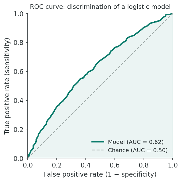
Discrimination is most often summarised by the area under the receiver operating characteristic (ROC) curve (Hanley & McNeil, 1982; Wikipedia, n.d.), while calibration assesses agreement between predicted and observed risks (Steyerberg et al., 2010).

Selecting a cutpoint involves a trade-off between sensitivity and specificity. A lower cutpoint increases sensitivity but decreases specificity, and vice versa. The ROC curve provides a visual summary of this trade-off across all possible cutpoints.

Overdispersion

Pseudo-R² and Influential Observations

Pseudo-R² measures (e.g., McFadden’s, Cox-Snell, Nagelkerke) provide an indication of how much of the variation in the outcome is explained by the model. They are analogues of R² in linear regression but are not directly comparable. Values tend to be lower for logistic regression than for linear regression.

Influential observations can be identified using several diagnostic measures: outliers (large residuals), leverage (unusual covariate patterns), delta-betas (influence on individual coefficients), delta-χ², and delta-deviance (influence on overall fit). These diagnostics help identify observations that disproportionately affect the model.

Introduction and Overview

Sections 1–3 covered standard logistic regression. Section 4 places it in a wider context. Logistic regression is one example of the generalised linear model (GLM) family, which also includes the linear, Poisson, and other regressions you'll meet later in this course. The section closes with exact logistic regression, the small-sample alternative when standard maximum-likelihood methods fail.

Generalised Linear Models (GLMs)

Logistic regression is a member of the broader family of Generalised Linear Models (GLMs). A GLM is defined by two key components: (1) a link function that relates the expected value of the outcome to the linear combination of predictors, and (2) the distribution of the outcome variable.

The canonical link is the “natural” link function for each distribution. For binary data, the canonical link is the logit. Non-canonical links (e.g., probit, complementary log-log for binary data) can also be used. GLMs are estimated using maximum likelihood, often with iterative algorithms such as Newton-Raphson or iteratively reweighted least squares. Quasi-likelihood estimation can be used when the full distribution is not specified, requiring only the mean-variance relationship.

Exact Logistic Regression

Standard logistic regression relies on large-sample approximations. When the dataset is very small or severely unbalanced (e.g., very few events), these approximations may be poor, and ML estimates can be biased or fail to converge. Exact logistic regression uses conditional maximum likelihood to produce exact P-values and confidence intervals without relying on large-sample theory. A widely used alternative is the penalised-likelihood approach of Firth (1993), which reduces small-sample bias and handles separation gracefully.

Bringing It All Together

This lesson took the binary outcome — the most common outcome in epidemiology — and built a regression framework around it, building on the foundational work of David Cox (Wikipedia, n.d.; Cox, 1958). We started by showing why ordinary linear regression breaks for dichotomous data and how the logit transformation rescues us, then moved through coefficient interpretation as adjusted odds ratios, the assumption of linearity on the logit scale, and the likelihood-ratio and Wald tests for inference. Section 3 broadened the lens from estimation to evaluation: residuals, Hosmer–Lemeshow, ROC curves, calibration, pseudo-R², and overdispersion give complementary views of whether a fitted model is actually fit for purpose.

Section 4 placed logistic regression inside the wider GLM family and flagged the small-sample escape hatches — exact logistic regression for sparse data and perfect prediction, and conditional logistic regression for matched case-control studies. With those pieces in place you have the binary toolbox you'll keep using for the rest of the course: every later model in HSCI 410 (ordinal, multinomial, Poisson, Cox) is a variation on the same maximum-likelihood theme you have just learned.

The final assessment asks you to move fluently between the log-odds scale and the odds-ratio scale, and to choose appropriate diagnostics for a model someone hands you. Treat the questions like a code review of your own analytic habits.