n
0
Exploratory Data Analysis For Epidemiology
This course was developed by Dr. Kiffer G. Card, Faculty of Health Sciences, Simon Fraser University based on Dohoo, I. R., Martin, S. W., & Stryhn, H. (2012). Methods in Epidemiologic Research. VER Inc.
📚 Reference page, available throughout the lesson
This glossary collects the key concepts, people, and ideas you will meet in this lesson. Use it as a reference while you work through the material, or as a review before assessments. Type in the search box to filter entries.
Earlier lessons produced a clean, descriptive view of the data. This lesson takes the next step from description to inference: linear regression is the workhorse model for explaining or predicting a continuous outcome from one or more predictors, fit by ordinary least squares (Stigler, 1981). Across four content sections we walk through this in order: the simple and multivariable model and what its coefficients mean (this section), the ANOVA decomposition and how to test the model and its individual coefficients (a later section), how to handle different types of predictor variables and detect collinearity (a later section), and how to detect and model interactions and give a regression a defensible causal interpretation (a later section). Model diagnostics, the residual and influence checks that show whether the fit can be trusted, run alongside the R work throughout.
Up to this point, most examples of relating an outcome to an exposure have been based on qualitative outcome variables, that is, variables that are categorical or dichotomous. Linear regression is suitable for modelling the outcome when it is measured on a continuous or near-continuous scale. Examples include birth weight, blood pressure, body mass index, and disease frequency at a regional level.
In regression analysis, the relationship between the outcome and the predictors is asymmetric: we think the value of the outcome is caused by (or we wish to predict it by) the value of another variable (the predictor). Using X-variables to predict Y does not necessarily imply causation; we might just be estimating predictive associations.
When only one predictor variable is used, the model is called a simple regression model. The term “model” denotes the formal statistical formula that describes the relationship between the predictor and the outcome.
Springs, residuals, and the line that minimizes them. Next ▶ advances scenes.
A 6-scene visualization of OLS: scattered observations, a wobbling candidate line, residuals as physical springs, and the line settling into the unique position that minimizes the sum of squared errors.
In this equation, β0 is the intercept (or constant), β1 is the regression coefficient, and ε is the error term. The errors are assumed to be normally and independently distributed (ε ~ N(0, σ²)). We estimate these errors by residuals, the difference between the observed value and the value predicted by the model.
Suppose the outcome Y is systolic blood pressure in mmHg and the predictor X1 is age in years, and the fitted line is Ŷ = 100 + 0.5 × age. The intercept of 100 is the model’s predicted blood pressure at age 0, which is only a mathematical anchor rather than a real value for a newborn. The slope of 0.5 is usually the part you care about: comparing two people whose ages differ by one year, the model predicts the older one has, on average, a systolic blood pressure about 0.5 mmHg higher, roughly 20 mmHg across a 40-year span. Read it as a comparison of averages between groups that differ in the predictor; it does not by itself describe what happens inside any one person over time.
Click anywhere on the chart to add a point. Click on an existing point to remove it. The least-squares line, residuals, R², and standard error of the slope update live. Add an extreme outlier and watch one observation drag the entire line (Cook, 1977; Belsley, Kuh, & Welsch, 1980).
Almost without exception, the regression models used by epidemiologists will contain more than one predictor variable. These are known as multiple regression or multivariable models.
Multivariate indicates 2 or more outcome variables; multivariable denotes more than 1 predictor. In epidemiology, we almost always mean multivariable models.
A major difference from simple regression is that in the multivariable model, β1 is an estimate of the effect of X1 on Y after controlling for the effects of X2. This is the key advantage of multivariable analysis: it accounts for confounding by extraneous variables.
In observational studies, incorporating more than one predictor almost always leads to a more complete understanding of how the outcome varies, and it decreases the chance that the regression coefficients for exposures of interest are biased by confounding variables. The βs are not biased by any variable included in the equation, but they can be biased if confounding variables are omitted from the equation.
Assuming we have not included intervening variables or effects of the outcome in our model, the βs are not confounded by any variable in the regression equation. However, from a causal perspective, if intervening variables are included, the coefficients do not estimate the causal effect. One can never be sure that there are no important unmeasured confounders that were omitted from the model.
A major trade-off in model-building is to avoid omitting necessary confounding variables while not including variables of little importance. Including too many unimportant variables increases the number of βs estimated and may lead to poor performance of the equation on future datasets. Also, having to measure unnecessary variables increases the cost of future work.
Picking up the cleaned phaa_survey_clean.csv from an earlier lesson, we will (1) test bivariate correlations, (2) inspect a correlation matrix for the numeric variables we plan to include in a model, and (3) fit a multivariable linear regression for systolic BP. The full annotated script is in r-activities/HSCI_410_Lesson_3_Linear_Regression.R.
# 0. Load the cleaned data + packages we will use ---------------------------
library(corrplot); library(regclass); library(caret)
phaa <- read.csv("phaa_survey_clean.csv", stringsAsFactors = FALSE)
# 1. Bivariate correlation between two numeric variables --------------------
cor.test(phaa$age, phaa$systolic_bp,
method = "pearson")
# 2. Correlation matrix + visual --------------------------------------------
keep_num <- c("age", "bmi", "systolic_bp", "diastolic_bp",
"phys_act_min", "discrimination_score",
"social_support_score", "dep_score", "anx_score")
cor_mat <- cor(phaa[, keep_num], use = "complete.obs")
round(cor_mat, 2)
corrplot(cor_mat, method = "color", type = "upper",
addCoef.col = "black", tl.col = "black", tl.srt = 45)
# 3. Set the reference level on a factor before fitting lm() ----------------
phaa$gender <- as.factor(phaa$gender)
phaa$gender <- relevel(phaa$gender, ref = "Woman")
# 4. Multivariable linear model for systolic BP -----------------------------
model_3 <- lm(systolic_bp ~ age + gender + smoker + bmi
+ dep_score + phys_act_min,
data = phaa)
summary(model_3)
confint(model_3)
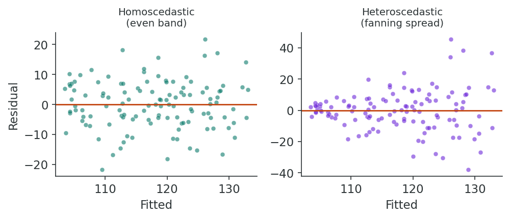
# 5. Diagnostics: linearity, equal variance, normal residuals, outliers -----
par(mfrow = c(2, 2)); plot(model_3); par(mfrow = c(1, 1))
VIF(model_3) # multicollinearity
varImp(model_3) # variable importanceHow to read the output. Each coefficient in summary(model_3) is the average change in systolic BP per one-unit increase in that predictor, holding the other predictors constant. The (Intercept) is the predicted BP when every numeric predictor is 0 and every factor is at its reference level, which is not always meaningful, which is why we centre age in a later lesson. VIF values > 5 mean two predictors are carrying mostly the same information.
Use the questions below to interpret the output you produced. Look at your console / plot before answering.
1. From cor.test(phaa$age, phaa$systolic_bp), what is the Pearson r and its 95% CI? Does the CI exclude zero? Translate the magnitude into plain English (small / moderate / strong).
2. In summary(model_3), what is the coefficient on age and its p-value? In one sentence, state the adjusted association of age and systolic BP, and whether the 95% CI from confint() excludes zero.
summary(model_3) typically shows an age coefficient of ~0.5 mmHg per year (range 0.3–0.7 depending on covariate inclusion) with p < 0.001 in a sample of n > 500. The 95% CI from confint() excludes zero. Adjusted association: each additional year of age is associated with roughly 0.5 mmHg higher systolic BP, after accounting for sex, BMI, and smoking. The effect compounds over age decades, explaining the ~15–20 mmHg average rise from age 30 to 70.3. Look at VIF(model_3). Which predictor has the highest VIF? Is it above 5 or 10? If you removed it, how would you expect the SE on a correlated predictor to change?
VIF(model_3) typically shows the highest VIF for one of the BP-related variables or BMI, usually around 2–3, below the conventional 5/10 thresholds. If a predictor with VIF > 5 were removed, the SE on its correlated counterpart would drop noticeably (typically by 15–30%), and the point estimate would shift slightly as the model re-attributes shared variance. Multicollinearity doesn't bias coefficients, but inflates their SEs and CIs, making true effects appear non-significant.1. What type of outcome variable is linear regression most suitable for?
2. In the equation Y = β0 + β1X1 + ε, what does β1 represent?
3. What is the key advantage of a multivariable regression model over a simple regression model?
Think of a continuous outcome variable in your field of interest. What predictors would you include in a regression model? How would you decide which variables are confounders versus intervening variables?
An earlier section set up the regression model. This section turns to the question of whether the model is doing useful work: how much of the variation in the outcome does it actually explain, and which individual coefficients are meaningfully different from zero? The ANOVA decomposition and the formal tests of model significance are how those questions get answered.
The idea behind regression is that information in the X-variables can be used to predict the value of Y. The formal way this is approached is to ascertain how much of the sums of squares (SS) of Y we can explain with knowledge of the X-variable(s).
| Source | Sums of Squares | df | Mean Square | F-test |
|---|---|---|---|---|
| Model (regression) | SSM = Σ(Ŷi − Ȳ)2 | dfM = k | MSM = SSM/dfM | MSM/MSE |
| Error (residual) | SSE = Σ(Yi − Ŷi)2 | dfE = n−(k+1) | MSE = SSE/dfE | |
| Total | SST = Σ(Yi − Ȳ)2 | dfT = n−1 | MST = SST/dfT |
Here, k is the number of predictor variables in the model (not counting the intercept). When the SS are divided by their degrees of freedom (df), the result is a mean square, denoted MSM (model), MSE (error), and MST (total). The MSE is our estimate of the error variance σ², and the square root of σ² is called the root MSE or the standard error of prediction.
We use the F-test from the ANOVA table to assess whether the predictors collectively have a statistically significant relationship with the outcome. The null hypothesis is H0: β1 = β2 = … = βk = 0.
In plain terms, the overall F-test asks a single yes-or-no question: taken as a set, do the predictors track the outcome better than simply predicting its overall mean for everyone? If the answer is no, the F ratio sits near 1; a large F with a small p-value says the predictors are doing real work.
A simple linear regression model with birth weight (-bwt-) as the outcome and gestation length (-gest-) as the sole predictor was fit using the bw5k dataset (n = 5,000).
Results: F(1, 4998) = 1,790.09, P < 0.0001, R² = 0.2637. The coefficient for -gest- is 124.5 gm per week (95% CI: 118.7–130.3), meaning for each additional week of gestation, birth weight increases by approximately 124.5 gm.
A t-test with n−(k+1) degrees of freedom is used to evaluate the significance of any individual regression coefficient. The usual null hypothesis is H0: βj = 0.
Two sources of uncertainty stack when you use a fitted model to predict. The first is uncertainty about where the regression line itself sits, captured by the usual standard error. The second is the natural scatter of an individual observation around that line. A confidence interval for the mean of Y at a chosen value x* uses only the first source: Ŷ ± t.05·SE. A prediction interval for a single new individual adds the second source, so it is always wider than the confidence interval. Both intervals widen as x* moves further from the mean of X1, because the line is pinned down most tightly near the centre of the data.
R² (the coefficient of determination) describes the amount of variance in the outcome “explained” by the predictor variables. One formula: R² = SSM/SST = 1 − (SSE/SST). Unfortunately, R² always increases as variables are added to the model. The adjusted R² = 1 − (MSE/MST) adjusts for the number of predictors and is useful for comparing models with different numbers of variables.
Sometimes it is necessary to simultaneously evaluate the significance of a group of X-variables (e.g., a set of indicator variables for a nominal variable). We compare the SSE of the full model with the SSE of the reduced model (without the group) using a partial F-test. This tells us whether the set of variables as a group contributes significantly to the model.
The F-test has a straightforward interpretation only when the X-variables are manipulated treatments in a controlled experiment. In observational studies, the F-statistic is influenced by the number of variables available, their correlations, the total number of subjects, and the method used for variable selection. Most variable selection methods tend to maximise F, meaning the observed F overestimates the actual significance of the model.
Run hundreds of simulated studies. Each study fits a regression of Y on X with a chosen true effect and sample size. Watch the distribution of p-values build up. With no real effect, p-values are uniform on [0,1]. With a real effect, p-values pile up near zero. Power = the proportion below α.
A scatter of n points; black line = OLS fit; t-statistic and p-value displayed.
Histogram of all p-values run so far. Red region = p < α (significant).
1. What does the F-test in the ANOVA table assess?
2. What does R² (the coefficient of determination) measure?
3. Why is adjusted R² preferred over R² when comparing models with different numbers of predictors?
Consider a regression model you have seen in published research or coursework. How would you interpret the R² value? What does a low R² mean practically, and does it necessarily indicate a poor model?
An earlier section evaluated the model's overall fit. This section turns to a practical question that often determines whether your model gives sensible answers: are your predictors entered correctly? Continuous, categorical, indicator, and polynomial predictors all need different handling, and highly correlated predictors (multicollinearity) can destabilize coefficient estimates without obvious warning signs.
The X-variables can be continuous or categorical. Categorical variables can be either nominal (levels with no meaningful numerical representation, e.g., race or city of residence) or ordinal (ordered levels, e.g., severity: low, medium, high). Nominal and ordinal variables with more than 2 levels must be converted to indicator variables before entering the regression.
Often the predictor variables have a limited range of possible or sensible values. For example, if gestation length is a predictor, the intercept reflects birth weight at 0 weeks, which is meaningless. It is useful to scale these variables by subtracting the lowest possible sensible value (or the average) before entering them into the model. This makes the intercept interpretable without changing the regression coefficient or its SE.
Example: Subtracting 39 weeks (the average gestation length) from -gest- gives gest39 = gest − 39. Now β0 reflects birth weight for a 39-week gestation (3,341 gm), a much more meaningful value than the original constant of −1,514 gm.
Indicator variables (also called dummy variables) are created variables whose values have no direct physical relationship to the characteristic being described. For a nominal variable with j levels, we need j − 1 indicator variables. The omitted level becomes the referent (comparison) category.
Example: For mother’s race with 3 categories, we create 2 indicator variables (X1 and X2). Race 3 (with both indicators = 0) becomes the referent. β1 estimates the difference in outcome between races 1 and 3, while β2 estimates the difference between races 2 and 3.
If the predictor variables are ordinal in type (reflecting relative changes in an underlying characteristic), hierarchical indicator variables are often preferred. These contrast the outcome in each level against the level immediately preceding it (assuming all hierarchical variables are in the model).
Example: For mother’s education (4 levels), the disjoint indicators compare each level to the lowest (baseline). The hierarchical indicators instead show: the coefficient for level 4 reflects the difference between level 3 (some college) and level 4 (university degree), showing the incremental effect of each step up in education.
| Variable | Indicator Coding | Hierarchical Coding |
|---|---|---|
| meduc_c4=2 (high school diploma) | 20.046 | 20.046 |
| meduc_c4=3 (some college) | 53.270 | 33.224 |
| meduc_c4=4 (university degree) | 80.599 | 27.329 |
If the predictor variables are too highly correlated, a number of problems arise. The estimated effect of each variable depends on the other predictors in the model. With highly correlated predictors, the βs will be highly and negatively correlated, and in extreme cases none of the individual coefficients will be significantly different from zero despite a significant overall F-test.
When a quadratic term (-gest_sq-) was added to a model already containing -gest-, the correlation between the two was 0.99, giving a VIF of 131. The SE of -gest- increased over 11 times (from 2.94 to 32.99). Centring -gest- by subtracting 39 (the mean) reduced the VIF from 131 to just 1.54 and the SE back down to 3.58.
1. For a nominal variable with 4 categories, how many indicator (dummy) variables are needed?
2. What does a VIF value greater than 10 suggest?
3. What is the primary purpose of centring a continuous variable before adding it to a regression model?
Why might highly correlated predictor variables cause problems in a multivariable regression model? What strategies would you use to detect and address collinearity in your own analyses?
Earlier sections set up a model with main effects only. This section takes two final design steps: testing whether the effect of one predictor depends on another (interaction) and giving the resulting coefficients a defensible causal interpretation. Both push linear regression beyond a curve-fitting exercise into a tool for answering causal questions, anchored in the DAG-based framework you met in an earlier lesson.
Given the component cause model, we might expect to see interaction when 2 factors act synergistically or antagonistically. In previous sections, models contained only main effects, assuming the association of X1 to Y is the same at all levels of X2. An interaction term tests whether the effect of one variable depends on the level of another.
We assess interaction by testing whether β3 = 0. If the interaction is absent (i.e., β3 is not significantly different from 0), the main effects (additive) model is deemed adequate. If the interaction is needed, centring becomes useful because it allows us to interpret β1 and β2 as linear effects when the centred version of the other variable is zero.
Example 14.9: The dichotomous versions of maternal weight gain (wtgain_c2: <30 lb vs ≥30 lb) and total birth order (tbo_c2: primiparous vs multiparous) were evaluated. The main effects model showed both factors were significant. Adding the interaction term (wg_c2*tbo_c2) revealed a significant interaction (β3 = −88.4, P = 0.010).
This means the positive effect of multiparous birth on birth weight is present if weight gain is low, but is negligible if weight gain is high. Similarly, high weight gain has a bigger effect in primiparous births (227 gm) than in multiparous births (139 gm).
Interactions involving categorical variables (with more than 2 levels) are modelled by including products between all indicator variables needed in the main effects model. For example, the interaction between a 3-level and a 4-level categorical variable requires (3−1) × (4−1) = 6 product variables. These 6 variables should be tested and explored as a group using the partial F-test.
In many multivariable analyses, the number of possibilities for interaction is large and there is no single correct way to assess if interaction is present. Unless the potential number of interactions is small, interactions should be limited to those of biological relevance. It is generally recommended that 3- and 4-way interactions only be investigated when there are good, biologically sound reasons for doing so.
So far, we have focused on the technical interpretation of regression coefficients. When making causal inferences, extra care is needed to ensure that only the appropriate variables are included in the analysis. A causal diagram is very helpful in this regard.
If a variable is an intervening variable (on the causal pathway between exposure and outcome), including it in the model will change the interpretation (Greenland, Pearl, & Robins, 1999). For example, if gestation length is an intervening variable between cigarette smoking and birth weight, including -gest- in the model adjusts away part of the causal effect of smoking. The total effect of smoking would be obtained from a model without -gest-, while the direct effect (not mediated through gestation) would require including it.
Our objective is to evaluate the effects of cigarette smoking (-cig-) on birth weight (-bwt-). The causal diagram indicates that gestation length (-gest-) is an intervening variable between -cig- and -bwt-. Consequently, -gest- and -wtgain- should be excluded from the model when estimating the total causal effect of smoking on birth weight.
The model includes: -white- (potential confounder), -college- (potential confounder), and -cig_2- (the exposure of interest). The interaction between -cig_2- and -white- was assessed.
1. What does a significant interaction term (β3) in a regression model indicate?
2. When estimating the total causal effect of an exposure, what should you do with intervening variables?
3. What tool is recommended before building a multivariable model to help distinguish confounders from intervening variables?
Consider an exposure–outcome relationship you are interested in. Draw (or describe) a causal diagram identifying potential confounders and intervening variables. How would the choice of which variables to include affect your estimate of the causal effect?
This lesson took the dataset you cleaned in an earlier lesson and built a working linear regression around it. An earlier section introduced the simple and multivariable model and made clear how each coefficient should be read. An earlier section used the ANOVA decomposition to ask whether the model is doing useful work, and the t-tests and confidence intervals to ask the same question of each coefficient. An earlier section dealt with the messiness of real predictors: scaling continuous variables, dummy-coding categorical ones, building hierarchical indicators, and using VIF to spot the collinearity that quietly destabilises coefficients. An earlier section closed the loop by adding interactions and giving the fitted model a defensible causal reading via a DAG.
The lesson treats linear regression as an inferential tool rather than a line through points: its coefficients carry meaning only when the predictors have been entered correctly, the assumptions have been checked, and the causal structure has been laid out in advance. A later lesson picks up directly from here with the question of which predictors should enter the model in the first place, the model-building strategies that turn the machinery of this lesson into a defensible final analysis.
The final assessment below covers all material from this lesson. You must answer all 15 questions correctly (100%) and complete the final reflection to finish the lesson.
Reflect on the full chapter. How does linear regression differ from the categorical outcome methods you have previously studied? In what situations would you choose linear regression, and what are the key assumptions you need to verify before trusting your results?
1. Linear regression is most appropriate when the outcome variable is:
2. In the simple regression model Y = β0 + β1X1 + ε, what does β0 represent?
3. Residuals in a regression model are:
4. In a multivariable model, β1 represents the effect of X1 on Y:
5. The root MSE (root mean square error) in a regression model is:
6. The null hypothesis for the overall F-test in regression is:
7. If R² = 0.26 in a regression model, what can we conclude?
8. Why should we use adjusted R² rather than R² when comparing models?
9. To code a nominal variable with 5 categories for regression, you would create:
10. What is the purpose of scaling a predictor variable (e.g., subtracting the mean)?
11. A VIF of 1.0 for a predictor indicates that:
12. In the model Y = β0 + β1X1 + β2X2 + β3X1*X2 + ε, a significant β3 indicates:
13. Including an intervening variable in a causal regression model will:
14. The regression coefficient for a dichotomous predictor (coded 0/1) represents:
15. Ignoring measurement errors in predictor variables tends to:
✦ Before submitting: pass every section knowledge check (100%) and complete every reflection.