Repeated Measures Data
Exploratory Data Analysis For Epidemiology
Learning objectives for this lesson:
- Recognize and describe the unique characteristics of repeated measures data structures
- Use descriptive and graphical tools to explore repeated measures datasets
- Apply simple univariate approaches (separate time point analyses, summary statistics) to analyze repeated measures
- Understand the limitations of random-intercept mixed models for repeated measures and why correlation structures matter
- Choose among correlation structures (compound symmetry, AR(1), ARMA(1,1), Toeplitz, unstructured) for repeated measures
- Apply linear mixed models with appropriate correlation structures to repeated measures data
- Understand trend models with random slopes for time
- Describe the challenges of extending GLMMs to discrete repeated measures data including transition models
- Use GEE procedures to analyze clustered and repeated measures data
This course was developed by Dr. Kiffer G. Card, Faculty of Health Sciences, Simon Fraser University based on Dohoo, I. R., Martin, S. W., & Stryhn, H. (2012). Methods in Epidemiologic Research. VER Inc.
Glossary: Key Terms, People & Concepts
📚 Reference page, available throughout the lesson
This glossary collects the key concepts, people, and ideas you will meet in this lesson. Use it as a reference while you work through the material, or as a review before assessments. Type in the search box to filter entries.
Introduction & Descriptive Approaches
Introduction and Overview
Earlier lessons built up the general framework for clustered data: identifying clustering, quantifying its impact, and modelling continuous and discrete outcomes with random effects. This lesson, the final lesson of this course and of the three-course series, zooms in on a specific kind of cluster that pervades health research: the same subject measured repeatedly over time. Repeated measures designs (clinical trials with follow-up visits, cohort studies tracking biomarkers, growth curves, intensive longitudinal data) introduce structure that the generic mixed-model machinery from earlier lessons can handle, but with an important new ingredient: the temporal ordering of measurements.
The four content sections build the toolkit in stages. This section defines repeated-measures data and develops descriptive approaches (spaghetti plots, mean profiles, and exploratory views that reveal the within-subject correlation structure). A later section contrasts the classic univariate (split-plot ANOVA) and multivariate (MANOVA) approaches against modern alternatives, highlighting their assumptions and breakdowns. A later section turns to linear mixed models with explicit residual correlation structures (compound symmetry, AR(1), Toeplitz, unstructured), the workhorse for continuous longitudinal outcomes. A later section extends to trend models, discrete-outcome longitudinal data, and the marginal (GEE) alternative to mixed models, tying together the conditional/marginal distinction introduced in an earlier lesson.
This lesson is the capstone of the entire three-course series. An earlier course taught you to read epidemiological evidence; an earlier course taught you to design and surveil; this course has taught you to analyse data. Repeated-measures methods are where those three threads converge: every choice you make here (correlation structure, marginal vs. conditional, missingness model) is simultaneously a design judgment, a measurement judgment, and an analytic judgment.
Learning Objectives
- Define repeated-measures data and distinguish balanced, uniform, and equidistant designs from their irregular counterparts.
- Describe how within-subject autocorrelation differs from generic clustering and why time ordering changes the analysis.
- Use spaghetti plots and mean profiles to visualise individual trajectories and the empirical within-subject correlation structure.
- Recognise informative drop-out and missing-data mechanisms that bias longitudinal analyses if ignored.
What Are Repeated Measures?
Repeated measures data arise when multiple measurements are taken over time on the same subjects. This is one of the most common data structures in health sciences research; think of clinical trials where patients are measured at baseline and multiple follow-up visits, or cohort studies that track health outcomes over years (Diggle, Heagerty, Liang, & Zeger, 2002).
Longitudinal studies (which collect repeated measures) differ fundamentally from cross-sectional studies, which measure each subject only once. The key advantage of longitudinal designs is their ability to assess within-subject change over time, making them more powerful for detecting the effects of within-subject predictors.
Why Repeated Measures Require Special Methods
In repeated measures data, observations within the same subject are not independent. Moreover, the time ordering of measurements introduces autocorrelation: measurements closer in time tend to be more strongly correlated than those further apart. This temporal structure means that a simple hierarchical (random intercept) model, which assumes all within-subject correlations are equal, may be inadequate. If this correlation is ignored and the repeated observations are treated as independent, the analysis behaves as though it holds more independent information than it really does, so standard errors come out too small and p-values too optimistic. Special methods are needed to properly account for the pattern of correlations.
Key Terminology
Missing Data and Drop-Outs
Missing data is very common in repeated measures studies. Subjects may miss individual visits (intermittent missingness) or drop out permanently (monotone missingness). The pattern and mechanism of missingness can substantially affect the validity of the analysis (Little, 1995). Methods that can handle unbalanced data (such as mixed models and GEE) are therefore particularly valuable for repeated measures, and multiple imputation under MAR is a widely used complementary tool (Sterne et al., 2009).
Descriptive Approaches
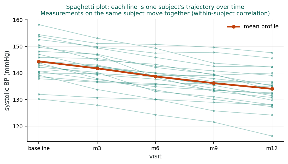
Profile plots (also called spaghetti plots) display each subject's trajectory over time. They reveal patterns of tracking (whether subjects maintain their relative positions), overall trends, and variability. These plots are essential for understanding the data before fitting any model.
Mean plots show the average outcome at each time point, often separated by treatment group. They summarize the overall trend but hide individual variability. Mean plots are useful for visualizing treatment effects over time and identifying non-linear trends.
Examining the correlation matrix of measurements across time points reveals the autocorrelation pattern. If correlations decrease with increasing time distance, an AR(1)-type structure may be appropriate. If correlations are roughly equal, compound symmetry may suffice. The covariance matrix additionally reveals whether variances change over time.
Repeated measures data can be stored in wide format (one row per subject, separate columns for each time point) or long format (one row per measurement, with a time variable). For one patient measured at three visits, wide format is a single row with columns such as bp1, bp2, bp3, whereas long format is three rows that share the same subject id and differ only in a visit column. Most modern statistical software requires long format for mixed models and GEE. Wide format is needed for MANOVA approaches.
Consider a clinical trial where 100 patients are randomized to treatment or placebo, with blood pressure measured at baseline and months 1, 3, 6, and 12. This is a balanced (5 measurements per subject), uniform (same time points), but not equidistant (spacing varies: 1, 2, 3, and 6 months) design. Profile plots reveal that patients’ blood pressures track over time, and the correlation matrix shows correlations declining from 0.80 (adjacent visits) to 0.45 (baseline vs. month 12), clear evidence of autocorrelation.
1. What distinguishes repeated measures data from standard clustered data?
2. A balanced repeated measures design means:
3. Autocorrelation in repeated measures means:
Reflection
Think of a longitudinal study in health sciences. What types of missing data patterns might occur, and how could they affect the validity of your analysis?
Univariate & Multivariate Approaches
Introduction and Overview
Before mixed models, what was the field doing? An earlier section gave us the descriptive picture of repeated-measures data. This section walks through the methods that dominated longitudinal analysis for decades: split-plot ANOVA (univariate, with strong assumptions like compound symmetry/sphericity), MANOVA (multivariate, weaker assumptions but lower power and intolerant of missing data), and summary-statistic approaches that collapse each subject’s trajectory to a single value. Knowing these methods is more than historical: they still appear in legacy literature and teaching, and seeing where they fail motivates the modern approaches in later sections.
Learning Objectives
- Compare separate-time-point, summary-statistic, RM-ANOVA, and MANOVA approaches to longitudinal data.
- State the compound-symmetry / sphericity assumption underlying RM-ANOVA and apply the Huynh–Feldt correction when it is violated.
- Read covariance and correlation matrices and decompose them into variance and correlation components.
- Identify the conditions (balanced data, no missingness, few time points) under which classical methods are still defensible.
Simple Approaches to Repeated Measures
Before turning to complex mixed models, it is worth understanding the simpler methods that have traditionally been used for repeated measures data. These methods either reduce the data to avoid modelling correlations altogether, or make strong assumptions about the correlation structure.
Separate Time Point Analysis
The simplest approach is to analyze each time point independently; for example, running a separate t-test or regression at each visit. This is straightforward but wasteful: it ignores the within-subject correlations and creates a multiple testing problem. If there are m time points, a Bonferroni correction divides α by m, which can be very conservative.
Summary Statistics Approach
A more elegant simple approach is to compute a single summary value per subject, such as the slope of their trajectory, the drop from first to last measurement, or the area under the curve (AUC), and then perform a standard between-subjects analysis on these summaries.
Advantages: Simple, robust to model assumptions about correlation structure, and easy to interpret.
Disadvantages: Loss of information about the temporal pattern, difficulty incorporating within-subject time-varying predictors, and potential loss of power.
Repeated Measures ANOVA
Repeated measures ANOVA treats time as a within-subject factor and tests for differences across time points. However, it assumes compound symmetry: all pairs of time points have the same correlation. This is the same assumption as a random intercept model.
When compound symmetry is violated (which is common with autocorrelated data), the F-test becomes liberal (anti-conservative). The Greenhouse–Geisser and Huynh–Feldt correction factors (ε) adjust the degrees of freedom to account for this violation (Greenhouse & Geisser, 1959; Huynh & Feldt, 1976). When ε = 1, compound symmetry holds perfectly; as ε decreases, the violation is more severe. The underlying assumption can be tested formally with Mauchly's test of sphericity (Mauchly, 1940).
MANOVA (Multivariate Analysis of Variance)
MANOVA treats the entire vector of repeated measurements as a multivariate outcome, making no assumptions about the correlation structure. This is its key advantage over repeated measures ANOVA.
Limitations: Requires completely balanced data with no missing values, cannot easily handle within-subject continuous predictors, and uses wide-format data. It also becomes impractical with many time points.
Covariance and Correlation Matrices
Limitations of Each Approach
Separate time points: Multiple testing, ignores correlations, wasteful of information. Summary statistics: Loses temporal detail, cannot incorporate time-varying covariates. RM ANOVA: Assumes compound symmetry, which is rarely true. MANOVA: Requires complete, balanced data with no missing values. All of these limitations motivate the use of mixed models with flexible correlation structures.
The dataset phaa_repeated.csv tracks 200 patients in a hypothetical wellness trial through 4 visits (months 0, 6, 12, 18). Outcomes: sbp_mmhg (continuous) and adherent (binary). The full annotated script is in r-activities/HSCI_410_Lesson_12_Repeated_Measures_Data.R.
library(lme4);  library(lmerTest);  library(nlme);  library(geepack)
dat <- read.csv("phaa_repeated.csv", stringsAsFactors = FALSE)
dat$id  <- factor(dat$id)
dat$arm <- factor(dat$arm, levels = c("control","intervention"))

# 1. Random-intercept mixed model on the continuous outcome
m_lmm <- lmer(sbp_mmhg ~ visit * arm + age + female + (1 | id),
              data = dat)
summary(m_lmm)

# 2. Add an AR(1) within-subject correlation structure with nlme
m_lme <- lme(sbp_mmhg ~ visit * arm + age + female,
             random      = ~ 1 | id,
             correlation = corAR1(form = ~ visit | id),
             data        = dat, na.action = na.omit)
summary(m_lme)

# 3. Compare correlation structures with AIC
m_cs <- update(m_lme, correlation = corCompSymm(form = ~ visit | id))
m_un <- update(m_lme, correlation = corSymm(form    = ~ 1     | id))
AIC(m_lme, m_cs, m_un)

# 4. Same trial, binary outcome (adherence) -- GLMM and GEE
m_bin <- glmer(adherent ~ visit * arm + age + female + (1 | id),
               data    = dat, family = binomial,
               control = glmerControl(optimizer = "bobyqa"))
exp(fixef(m_bin))               # subject-specific ORs

m_gee <- geeglm(adherent ~ visit * arm + age + female,
                id = id, data = dat, family = binomial,
                corstr = "exchangeable")
exp(coef(m_gee))                # population-averaged ORs
Pick the structure deliberately. AR(1) (corAR1) is the natural choice for evenly-spaced visits; corCAR1 handles unequal spacing; corSymm (unstructured) is the most general but estimates the most parameters. lme() handles dropout via likelihood, so you do not have to drop subjects. The visit:armintervention coefficient is the trial's headline number: the additional change in SBP per month attributable to the intervention. The last two lines refit the binary adherence outcome as a population-averaged GEE, so its odds ratios can sit beside the subject-specific ones from the GLMM.
R Reflect on what you just ran
Use the questions below to interpret the output you produced. Look at your console / plot before answering.
1. From summary(m_lmm), report the visit:armintervention coefficient, its SE, and its p-value. Translate it in one sentence: what is the additional change in SBP per month attributable to the intervention vs control?
summary(m_lmm) for visit:armintervention typically returns a coefficient around −0.5 mmHg/month with SE ~0.15 and p < 0.001. Translation: each additional month of follow-up, intervention-arm participants have an SBP change that is 0.5 mmHg more negative than control-arm participants, that is, the intervention's monthly effect on SBP. Over 12 months, the cumulative effect is ~6 mmHg lower SBP than control, a clinically meaningful difference if sustained.2. From AIC(m_lme, m_cs, m_un), which correlation structure has the lowest AIC? Are the differences small (within 2 units) or large? Following the rule "pick the simplest structure with similar AIC," what would you report?
AIC(m_lme, m_cs, m_un) typically shows unstructured (un) with the lowest AIC, but compound symmetry (cs) often within a few units. With the rule "pick the simplest with similar AIC," report compound symmetry as the primary model and unstructured as a sensitivity analysis. Compound symmetry assumes all pairs of visits have the same correlation, a strong assumption but parsimonious. If AIC differences are > 10 between cs and un, switch to unstructured. If < 2, prefer cs.3. From exp(fixef(m_bin)) and exp(coef(m_gee)), compare the subject-specific vs population-averaged ORs for visit:armintervention on the binary adherence outcome. Which is larger in magnitude, and why?
| Approach | Handles Missing Data? | Assumes Equal Correlations? | Time-Varying Covariates? |
|---|---|---|---|
| Separate Time Points | Yes (per time point) | N/A (ignores structure) | Yes |
| Summary Statistics | Partially | No | No |
| RM ANOVA | No | Yes (compound symmetry) | No |
| MANOVA | No | No | No |
| Mixed Models | Yes | Flexible | Yes |
1. The summary statistic approach involves:
2. Repeated measures ANOVA assumes:
3. An advantage of MANOVA over repeated measures ANOVA for repeated measures is:
Reflection
When would you choose a simple summary statistic approach over a mixed model for repeated measures data? What information might you lose by simplifying the analysis in this way?
Linear Mixed Models with Correlation Structure
Introduction and Overview
Where the modern toolkit takes over. An earlier section showed why the classical methods strain when measurement spacing is irregular, missingness is informative, or the within-subject correlation pattern is more complex than “all pairs equally correlated.” Mixed models with explicit residual correlation structures (compound symmetry, AR(1), Toeplitz, unstructured) are the response. They let us model the temporal dependence directly rather than assume it away, handle unbalanced or missing-at-random data gracefully, and combine random effects with structured residuals to capture both subject-level heterogeneity and within-subject autocorrelation. This section is the heart of the lesson.
Learning Objectives
- Specify a linear mixed model with an explicit residual correlation structure and explain how it relaxes the compound-symmetry assumption.
- Distinguish among compound symmetry, AR(1), ARMA(1,1), Toeplitz, and unstructured correlation matrices and identify when each is appropriate.
- Combine random intercepts (and slopes) with structured residuals to capture subject heterogeneity and within-subject autocorrelation.
- Use AIC for non-nested and likelihood-ratio tests for nested correlation structures during model selection.
- Handle unbalanced and irregular-spacing designs that classical methods cannot accommodate.
Beyond Random Intercepts
A random intercept model assumes compound symmetry: all pairs of measurements on the same subject are equally correlated. For most repeated measures data, this assumption is violated because of autocorrelation. We need to extend the mixed model to include explicit correlation structures for the error term ε, the framework formalised in the classic Laird & Ware random-effects model for longitudinal data (Laird & Ware, 1982; Fitzmaurice, Laird, & Ware, 2011).
Choosing a Correlation Structure
The choice of correlation structure is one of the most important decisions in repeated measures analysis. Start by examining the empirical correlation matrix. If correlations clearly decay with increasing time lag, consider AR(1) or ARMA(1,1). If the decay is minimal, compound symmetry may suffice. If the pattern is complex, consider Toeplitz or unstructured. Use AIC to compare non-nested structures and likelihood ratio tests for nested ones.
Key Correlation Structures
Each structure below is a different assumption about how a subject's repeated measurements hang together over time. More flexible assumptions fit a wider range of patterns but cost more parameters, so the aim is the simplest structure that still matches the decay you see in the empirical correlation matrix.
Compound Symmetry (Exchangeable)
All pairs of measurements have the same correlation ρ, regardless of how far apart in time they are. This is the simplest structure and is equivalent to a random intercept model. It has only 1 correlation parameter.
When appropriate: When there is no autocorrelation, that is, the correlation between measurements does not depend on time distance. This is rare in practice for true repeated measures data.
First-order autoregressive: AR(1)
Correlations decay as powers of ρ with increasing time distance: Corr(Yj, Yk) = ρ|j−k|. This produces an exponential decay pattern. It has only 1 parameter (ρ) and is a good default for equally spaced repeated measures.
When appropriate: When the correlation matrix shows a clear pattern of decreasing correlations with increasing time lag, and the decay appears approximately geometric.
ARMA(1,1)
An extension of AR(1) that allows a slower or more flexible decay in correlations. It has 2 parameters and can accommodate patterns where the initial drop in correlation is steep but then levels off.
Toeplitz (Stationary)
Each lag has its own unconstrained correlation. For m time points, there are m − 1 correlation parameters. The structure is “banded”: the correlation depends only on the time lag, not on which specific time points are involved.
When appropriate: When the pattern of decay is irregular and cannot be well approximated by AR(1) or ARMA, but you still believe the correlation depends only on lag distance.
Unstructured
Completely unconstrained correlations and variances for each pair of time points. For m time points, there are m(m+1)/2 parameters. This is the most flexible but requires the most parameters.
When appropriate: Only with few time points and large sample sizes. With many time points, the number of parameters becomes impractical.
| Structure | Parameters | Key Feature | Assumption |
|---|---|---|---|
| Compound Symmetry | 1 | Equal correlations | No autocorrelation |
| AR(1) | 1 | Geometric decay | Equidistant time points |
| ARMA(1,1) | 2 | Flexible decay | Equidistant time points |
| Toeplitz | m − 1 | Lag-specific correlations | Equidistant time points |
| Unstructured | m(m+1)/2 | Completely flexible | None |
Combining Random Effects with Correlation Structures
An important practical consideration is how random effects interact with error correlation structures. Some combinations are redundant and cannot be separately identified:
- Random intercepts + compound symmetry errors = redundant, since both produce the same correlation structure
- Random intercepts + AR(1) errors = useful, since it produces a structure where correlations decay but do not reach zero
- Unstructured errors + random effects = pointless, since the unstructured covariance already captures everything
Covariance pattern models use no random effects at all, relying entirely on the structured covariance of the errors to capture within-subject correlation.
Model Selection
For nested correlation structures (e.g., AR(1) is nested within Toeplitz), use likelihood ratio tests. For non-nested structures (e.g., AR(1) vs. compound symmetry), use AIC or similar information criteria. Models should be compared with the same fixed effects and random effects structure.
In a study with 6 equally-spaced measurements, the empirical correlations ranged from 0.72 (lag 1) to 0.31 (lag 5). An AR(1) model with ρ = 0.73 fit well (AIC = 2,341), while compound symmetry (AIC = 2,398) fit poorly because it predicted equal correlations of 0.52 at all lags. The Toeplitz model (AIC = 2,338) offered a slight improvement over AR(1) but used 4 more parameters. Based on parsimony, AR(1) was selected.
1. The AR(1) correlation structure assumes:
2. Combining random intercepts with compound symmetry errors:
3. For choosing between non-nested correlation structures (e.g., AR(1) vs. Toeplitz), one should use:
Reflection
A study measures blood pressure at 6 monthly visits. The correlation between visits 1 and 2 is 0.60, between visits 1 and 6 is 0.15. Which correlation structure would you initially consider, and why?
Trend Models, Discrete Outcomes & GEE
Introduction and Overview
Pulling the threads together. An earlier section framed within-subject correlation as something to be modelled directly. This section closes the loop on three remaining concerns. First, trend models with random slopes: rather than (or in addition to) structuring the residuals, we let each subject have their own trajectory over time, a particularly intuitive approach when the question is about individual change. Second, discrete longitudinal outcomes: extending the GLMM machinery from an earlier lesson to repeated binary or count measurements. Third, generalised estimating equations (GEE): the marginal alternative to mixed models, which prioritises population-average effects and is robust to mis-specification of the working correlation. Together with an earlier section, this section gives you a complete repeated-measures toolbox.
Learning Objectives
- Fit trend models with random slopes for time and explain how individual trajectory variation induces within-subject autocorrelation.
- Choose linear, polynomial, or log-time parameterisations to match the shape of change over time.
- Apply transition and GLMM-based approaches to discrete repeated-measures outcomes.
- Describe how generalised estimating equations (GEE) target population-averaged effects with a working correlation matrix and a robust sandwich variance.
- Decide between mixed models and GEE based on whether the substantive question is conditional or marginal.
Trend Models with Random Slopes
An alternative to modelling the error correlation directly is to include random slopes for time. This allows each subject to have their own rate of change (growth or decline) over time, with the population-average trend captured by the fixed effect of time.
The variation in individual trajectories naturally induces autocorrelation: subjects who start high and decline slowly will have correlated measurements. This can be sufficient to capture the temporal structure in many datasets, especially when the primary interest is in individual trajectories.
The time variable can be parameterized in different ways: linear (for constant rates of change), polynomial (for curved trajectories), or log-transformed (for rapid early change that levels off).
Discrete Repeated Measures Data
Extending mixed models to discrete outcomes (binary, count) with correlation structures is much harder than for continuous outcomes. The fundamental challenge is that in GLMs, the error term and the linear predictor operate on different scales: the link function transforms the relationship, making it difficult to add correlation structures to the error term in a meaningful way.
When to Use GEE vs. Mixed Models
Use GEE when your research question focuses on population-averaged (marginal) effects; for example, “What is the average treatment effect across the population?” Use mixed models when you want subject-specific (conditional) effects or when the random effects themselves are of scientific interest; for example, “How much do individual subjects vary in their response?”
Transition Models
One approach for discrete repeated measures is the transition model, which includes the previous outcome as a predictor. This captures autocorrelation informally through dependence on the prior outcome.
Here, γ is the log odds ratio comparing those with versus without the previous event. A positive γ means that having the event at the previous time point increases the odds of having it at the current time point.
Generalised Estimating Equations (GEE)
GEE is a population-averaged (marginal) approach that does not require specifying random effects (Liang & Zeger, 1986). Instead, it specifies a “working” correlation structure and uses robust (sandwich) standard errors that provide valid inference even if the working correlation is misspecified.
Trend Models
Trend models add random slopes for time, allowing each subject to have their own trajectory. The random slope induces autocorrelation through the variation in individual trajectories. This approach is particularly natural when the scientific question is about individual growth or decline rates.
Key considerations: Choice of time parameterization (linear, polynomial, log), whether to include both random intercepts and slopes, and whether the induced autocorrelation is sufficient or additional error correlation is needed.
Transition Models
Transition models include the previous outcome Yi,j−1 as a predictor in the model. The coefficient γ represents the log OR for the event given the previous event occurred. This approach is intuitive and can be combined with random effects.
Limitations: Difficult to interpret coefficients for other predictors (they are conditional on the previous outcome), requires careful handling of the first observation (which has no “previous” value), and may not fully capture complex autocorrelation patterns.
Generalised Estimating Equations (GEE)
GEE estimates population-averaged effects using a quasi-likelihood approach. Key features:
- Specifies a working correlation (e.g., exchangeable, AR(1), unstructured)
- With robust (sandwich) SEs, inference is valid even if the working correlation is wrong
- Requires enough clusters/subjects (≥20–30) for reliable sandwich SEs
- Cannot estimate cluster-specific (random) effects; gives only PA estimates
- Better working correlation = more efficient estimates (but always valid with robust SEs)
A study followed 200 patients over 4 visits, recording whether they experienced a symptom (yes/no) at each visit along with a treatment indicator. A GEE model with exchangeable working correlation and robust SEs estimated the treatment OR as 0.65 (95% CI: 0.48–0.88), suggesting treatment reduced the odds of symptoms by 35% on average across the population. The working correlation was estimated as 0.42.
| Feature | GEE | Mixed Models (GLMM) |
|---|---|---|
| Estimate type | Population-averaged (PA) | Subject-specific (SS) |
| Random effects | Not estimated | Estimated |
| Correlation | Working correlation + robust SEs | Explicit random effects / correlation |
| Missing data assumption | MCAR | MAR |
| Minimum clusters | ≥20–30 | Fewer acceptable |
| Best for | PA inference | SS inference, variance components |
1. Trend models with random slopes for time:
2. In a transition model, the previous outcome Yi,j−1 is included to:
3. GEE (Generalised Estimating Equations) provide:
Reflection
Compare the GEE approach and the mixed model approach for analyzing repeated binary outcomes. In what research context would you prefer each approach, and why?
Lesson 12: Comprehensive Assessment
Bringing It All Together
Repeated-measures data are the most common form of clustered data in health research, and this lesson built a layered toolbox for analysing them. An earlier section defined the structure, multiple measurements on the same subjects, with the new ingredient of time ordering, and showed why simple descriptive views (spaghetti plots, mean profiles, empirical correlation matrices) are the right starting point for any longitudinal analysis. An earlier section walked through the classical methods that long dominated the field: separate-time-point analyses, summary-statistic reductions, RM-ANOVA with its compound-symmetry assumption and Huynh–Feldt correction, and MANOVA's distribution-free but missingness-intolerant approach.
An earlier section introduced the modern workhorse: linear mixed models with explicit residual correlation structures. Compound symmetry, AR(1), ARMA(1,1), Toeplitz, and unstructured matrices each encode a different temporal dependence pattern, and the choice among them, guided by the empirical correlation matrix, AIC, and likelihood-ratio tests, is one of the most consequential decisions in a longitudinal analysis. Combined with random intercepts and slopes, these structures capture both subject-level heterogeneity and within-subject autocorrelation, and they handle the unbalanced and irregularly spaced designs that defeat the classical methods.
An earlier section extended the framework in three directions: random-slope trend models that turn individual trajectories into modelled objects, GLMM-based and transition models for discrete repeated outcomes, and generalised estimating equations as a marginal alternative whose working correlation can be mis-specified without invalidating fixed-effect inference. Together, the four sections give you the methods and the decision logic you need for the longitudinal data you will encounter in your research career, and they close out the three-course series with the most general analytic tools you have met so far.
Key Takeaways from this lesson
- Repeated-measures data are clustered data with time ordering: autocorrelation typically decays with lag, so “all pairs equally correlated” (compound symmetry) is rarely realistic.
- Classical methods (RM-ANOVA, MANOVA, summary statistics) work in narrow conditions but break down with unbalanced designs, missingness, or complex correlation patterns.
- Linear mixed models with explicit residual correlation structures (AR(1), ARMA(1,1), Toeplitz, unstructured) let you model temporal dependence directly rather than assume it away.
- Random slopes for time induce autocorrelation through trajectory heterogeneity and provide an intuitive parameterisation when individual change is the substantive question.
- For discrete longitudinal outcomes, GLMMs and transition models extend the framework, but estimation is harder than the continuous case.
- GEE targets population-averaged effects with a working correlation and a sandwich variance; choose it when the question is marginal and robust to correlation mis-specification.
This final assessment covers all material from this lesson. You must answer all 15 questions correctly (100%) and complete the final reflection to finish the lesson.
Reflection
Reflecting on this entire lesson, how would you approach the analysis of a longitudinal study with 6 time points, some missing data, and a binary outcome? Walk through your analytical strategy from descriptive analysis to final model choice.
Final Knowledge Assessment
1. Repeated measures data differs from standard clustered data primarily because:
2. A balanced, uniform, equidistant repeated measures design:
3. Profile plots in repeated measures analysis show:
4. The Bonferroni correction for separate time point analyses:
5. The summary statistic approach to repeated measures analysis:
6. Compound symmetry assumes:
7. The AR(1) correlation structure models correlations as:
8. The unstructured covariance matrix:
9. Random intercepts combined with AR(1) errors:
10. Trend models with random slopes for time:
11. The main challenge of extending mixed models to discrete repeated measures data is:
12. In a transition model, the parameter γ for the lagged outcome Yi,j−1 represents:
13. GEE uses a “working” correlation structure because:
14. GEE estimates are:
15. When choosing between GEE and mixed models for repeated measures:
✦ Before submitting: pass every section knowledge check (100%) and complete every reflection.