Mixed Models for Discrete Data
Exploratory Data Analysis For Epidemiology
Learning objectives for this lesson:
- Understand the generalised linear mixed model (GLMM) framework for discrete outcomes
- Write and interpret logistic regression models with random effects
- Distinguish between subject-specific (SS) and population-averaged (PA) interpretations
- Calculate the median odds ratio (MOR) and latent variable ICC for binary outcomes
- Apply mixed models to count data using Poisson regression with random effects
- Understand estimation challenges in GLMMs including ML, quasi-likelihood, and Laplace approximation
- Extend mixed models to ordinal, multinomial, and other discrete outcome types
- Evaluate when different estimation methods are appropriate and their trade-offs
This course was developed by Dr. Kiffer G. Card, Faculty of Health Sciences, Simon Fraser University based on Dohoo, I. R., Martin, S. W., & Stryhn, H. (2012). Methods in Epidemiologic Research. VER Inc.
Glossary: Key Terms, People & Concepts
📚 Reference page, available throughout the lesson
This glossary collects the key concepts, people, and ideas you will meet in this lesson. Use it as a reference while you work through the material, or as a review before assessments. Type in the search box to filter entries.
Introduction & Logistic Regression with Random Effects
Introduction and Overview
An earlier lesson developed mixed models for continuous outcomes: random intercepts, random slopes, contextual effects, BLUPs, and diagnostics. This lesson extends every one of those ideas to discrete outcomes: binary (logistic), count (Poisson and negative binomial), ordinal, and multinomial. The framework you built last lesson carries over almost verbatim, but the link function, the likelihood, and the interpretation of effects all shift, and a new question becomes important: do you want a conditional (subject-specific) effect or a marginal (population-average) one?
The four content sections progress from the simplest extension to the practical realities of fitting and validating GLMMs. This section introduces the GLMM by way of logistic regression with a random intercept, the discrete analogue of the random-intercept linear mixed model. A later section generalises to count, ordinal, and categorical outcomes, and confronts the conditional-vs-marginal interpretation head on. A later section turns to estimation: penalised quasi-likelihood, Laplace approximation, adaptive Gauss–Hermite quadrature, MCMC, the menu of techniques used because no closed-form likelihood exists. A later section closes with inference, diagnostics, and a tour of related random-effects extensions (random-effects survival models, latent-variable formulations) that connect this lesson to the rest of the course.
Learning Objectives
- Specify a logistic GLMM with a random intercept and identify the role of the link function on the linear predictor.
- Distinguish subject-specific (conditional) from population-averaged (marginal) effects in non-linear mixed models.
- Apply the SS-to-PA conversion formula for logistic models and explain why the two coefficients differ.
- Interpret measures of cluster heterogeneity (median odds ratio, ICC on the latent scale) in a binary GLMM.
The Generalised Linear Mixed Model (GLMM)
Generalised linear mixed models (GLMMs) extend generalised linear models (GLMs) by adding random effects to the linear predictor (Stiratelli, Laird, & Ware, 1984; Breslow & Clayton, 1993). Just as linear mixed models allowed us to handle clustered continuous data, GLMMs handle clustered discrete data (binary, count, ordinal, and multinomial outcomes) while accounting for the correlation within clusters (Bolker et al., 2009).
Key Concept
The core idea of a GLMM is straightforward: take the linear predictor from a GLM and add random effects. For a logistic regression with a random intercept, the model becomes: logit(pij) = β0 + β1X1ij + ugroup(i), where ugroup(i) ~ N(0, σ²g). The random effect u captures between-cluster variation in the log-odds of the outcome.
Subject-Specific vs. Population-Averaged Interpretation
A critical distinction in GLMMs for discrete data is between subject-specific (SS) and population-averaged (PA) interpretations of the model parameters (Zeger, Liang, & Albert, 1988; Heagerty & Zeger, 2000). This distinction does not arise in linear mixed models but is fundamental for logistic and other non-linear models.
Because of the non-collapsibility of the odds ratio (averaging the odds ratio across clusters does not return the within-cluster odds ratio), SS coefficients are always larger in magnitude than PA coefficients. The approximate conversion formula is:
Consider a study of antibiotic resistance in cattle herds. A logistic GLMM with a random intercept for herd yields βSS = 0.85 for a treatment variable, with σ²g = 1.2. The SS odds ratio is exp(0.85) = 2.34: within any given herd, treatment more than doubles the odds of resistance. The median odds ratio (Larsen & Merlo, 2005) provides a complementary summary of between-herd heterogeneity.
Converting to PA: βPA ≈ 0.85 / √(1 + 0.346 × 1.2) = 0.85 / 1.19 = 0.71. The PA odds ratio is exp(0.71) = 2.03: across the population of herds, the average effect is smaller. The SS estimate is larger because it conditions on a specific cluster.
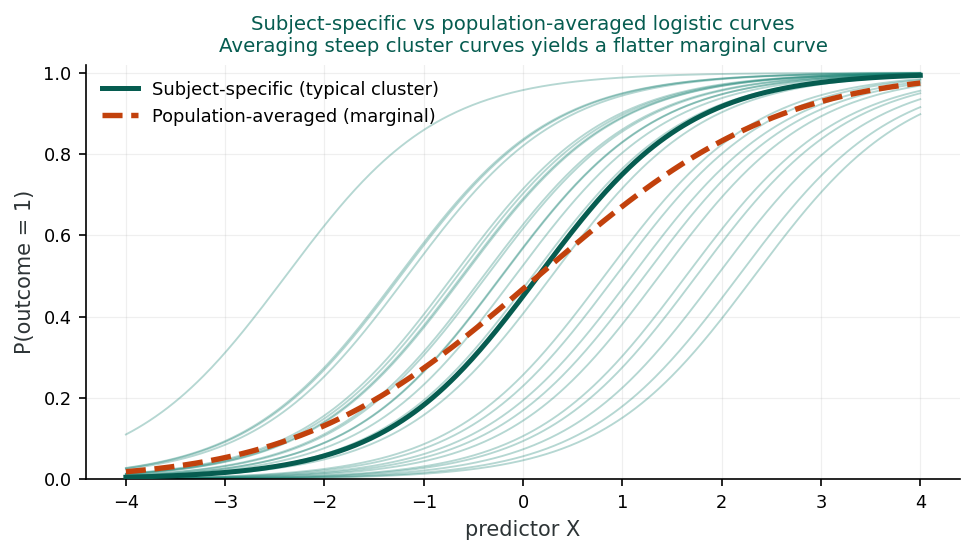
In plain words: which effect am I reading?
Picture one clinic. The subject-specific effect answers a within-clinic question: take two patients in that same clinic who differ only in the exposure, and ask how much their odds differ. The population-averaged effect answers a whole-population question: averaging across every clinic, how do the odds compare between exposed and unexposed people? The two numbers part ways because the logit curve is bent, and the average of a bent curve is not the same as the curve evaluated at the average. Averaging many steep subject-specific curves, each sitting at a different clinic's baseline, yields a gentler overall curve, so the population-averaged effect lands closer to no effect. A working rule: report the subject-specific effect when you advise one individual inside a known cluster, and the population-averaged effect when you plan for a whole population.
Measures of Cluster Heterogeneity
Median Odds Ratio (MOR)
The Median Odds Ratio quantifies between-cluster heterogeneity on the odds ratio scale. If you randomly select two clusters and compare a person from the higher-risk cluster to a person from the lower-risk cluster (with the same covariates), the MOR is the median of that odds ratio distribution.
An MOR of 1 means no between-cluster variation. Larger values indicate greater heterogeneity. The MOR allows direct comparison of the importance of cluster-level variation relative to fixed-effect odds ratios.
To make the scale concrete: an MOR of 2 means that if you pick two clusters at random and compare an otherwise-identical patient in each, the typical (median) ratio of their two odds is about 2, a gap as large as a moderately strong fixed-effect predictor. Reporting the MOR next to the fixed-effect odds ratios lets a reader judge whether where a patient is treated matters as much as the measured risk factors.
ICC for Binary Data
For binary outcomes, the latent variable ICC uses the fact that the individual-level variance on the logistic scale is π²/3 ≈ 3.29:
This provides an estimate of the proportion of total variance (on the latent scale) attributable to between-cluster differences.
The Latent Variable Approach
The binary outcome can be thought of as the result of thresholding a continuous latent variable. If the latent variable exceeds a threshold, the outcome is 1; otherwise, it is 0. In the logistic model, the individual-level error follows a standard logistic distribution with variance π²/3. This framework provides the basis for both the ICC calculation and the SS-to-PA conversion.
1. In a logistic GLMM, subject-specific (SS) coefficients are:
2. The Median Odds Ratio (MOR) measures:
3. The ICC for binary outcomes using the latent variable approach uses:
Reflection
Why does the distinction between subject-specific and population-averaged estimates matter in practice? Think of a scenario where you would prefer one interpretation over the other.
GLMMs for Count, Binary & Categorical Data
Introduction and Overview
From logistic to the full discrete-outcome family. An earlier section used logistic regression with a random intercept to introduce the GLMM. This section extends the framework outward to count outcomes (Poisson and negative binomial GLMMs, revisiting the count-data tools from an earlier lesson with clustering layered on top), ordinal outcomes (cumulative-link mixed models, an earlier lesson with random effects), and multinomial outcomes. Throughout, the conceptual difference between subject-specific and population-average effects becomes central: in non-linear models the two are not the same, and which one a stakeholder cares about should drive your modelling choice.
Learning Objectives
- Fit Poisson and negative-binomial GLMMs and interpret random effects as multiplicative cluster-level rate modifiers.
- Choose between normal and gamma random effects, and recognise when negative-binomial GLMMs handle residual overdispersion.
- Extend the GLMM framework to ordinal (cumulative-link mixed) and multinomial outcomes.
- Decide between conditional and marginal effects depending on the substantive question and stakeholder.
Poisson Regression with Random Effects
For count outcomes, Poisson regression with random effects models the log of the expected count as a function of predictors plus random effects:
Because the random effects enter on the log scale, they translate to multiplicative effects on the rate scale: μ = exp(Xβ) × exp(u). The group-level multipliers exp(u) follow a log-normal distribution when u is normally distributed.
Poisson with Normal Random Effects
The standard GLMM approach uses normally distributed random effects on the log scale. The group-level effects νgroup = exp(ugroup) are then log-normally distributed. This is the most common parameterisation in software.
This approach is flexible and can accommodate multiple levels of random effects, random slopes, and complex covariance structures, just like the linear mixed model framework.
Poisson with Log-Gamma Random Effects
An alternative parameterisation uses gamma-distributed random effects on the rate scale (equivalently, log-gamma on the log scale). When u follows a log-gamma distribution, the marginal distribution of counts has a convenient closed form.
This connection leads directly to the negative binomial distribution: a Poisson model with gamma-distributed rates yields negative binomial counts.
Negative Binomial as a Random Effects Model
The negative binomial distribution can be interpreted as a Poisson-gamma mixture: counts follow a Poisson distribution, but the rate varies across units according to a gamma distribution. This naturally accounts for overdispersion (variance > mean).
The negative binomial can be extended with additional random effects at higher levels, combining the overdispersion correction with explicit hierarchical structure.
| Model | Random Effect Distribution | Marginal Distribution | Key Feature |
|---|---|---|---|
| Poisson + Normal RE | Normal on log scale | No closed form | Standard GLMM; flexible |
| Poisson + Gamma RE | Gamma on rate scale | Negative binomial | Closed-form marginal |
| Negative Binomial | Implicit gamma | Negative binomial | Handles overdispersion |
The clustered dataset phaa_clinics.csv (carried forward from earlier lessons) has a binary outcome referred (1 = referred to a specialist). Same predictors as before but a binary outcome means a logistic GLMM. The full annotated script is in r-activities/HSCI_410_Lesson_11_Mixed_Models_for_Discrete_Data.R.
library(lme4);  library(performance);  library(geepack)
clinics <- read.csv("phaa_clinics.csv", stringsAsFactors = FALSE)
clinics$clinic_id    <- factor(clinics$clinic_id)
clinics$clinic_urban <- factor(clinics$clinic_urban,
                                  levels = c("rural","urban"))
clinics$smoker       <- factor(clinics$smoker, levels = c("No","Yes"))

# 1. Logistic GLMM (subject-specific)
m_glmm <- glmer(referred ~ age + female + smoker + bmi + clinic_urban
                            + (1 | clinic_id),
                data    = clinics,
                family  = binomial,
                control = glmerControl(optimizer = "bobyqa"))
summary(m_glmm)
exp(fixef(m_glmm))                     # subject-specific ORs
icc(m_glmm)                            # latent-scale ICC

# 2. GEE (population-averaged)
m_gee <- geeglm(referred ~ age + female + smoker + bmi + clinic_urban,
                id     = clinic_id, data = clinics,
                family = binomial, corstr = "exchangeable")
summary(m_gee)
exp(coef(m_gee))                       # population-averaged ORs

# 3. Compare side-by-side
cbind(GLMM_OR = exp(fixef(m_glmm)),
      GEE_OR  = exp(coef(m_gee)))
Subject-specific vs population-averaged. glmer() returns subject-specific ORs ("within the same clinic, two patients differ by ..."). GEE returns population-averaged ORs ("across the population, the average difference is ..."). For non-linear link functions like logit they are NOT the same; pick the one that matches your scientific question.
R Reflect on what you just ran
Use the questions below to interpret the output you produced. Look at your console / plot before answering.
1. From exp(fixef(m_glmm)) and exp(confint(m_glmm, method = "Wald")), report the subject-specific OR (and 95% CI) for smokerYes. Translate it into one sentence that explicitly conditions on the clinic (e.g., "within the same clinic, two patients...").
exp(fixef(m_glmm)) for smokerYes typically returns a subject-specific OR around 1.65, 95% CI roughly (1.30, 2.10). Interpretation, conditioning explicitly: within the same clinic, two patients who differ only in smoking status (one smoker, one non-smoker) differ in their odds of the outcome by a factor of about 1.65. This is a conditional, subject-specific effect: the comparison is between hypothetical patients in the same random-effect group.2. From icc(m_glmm), report the latent-scale ICC. Why does the binary ICC require a special formula (rather than just sigma^2_u / total variance like in linear mixed models)?
icc(m_glmm) typically returns a latent-scale ICC around 0.10–0.15. The binary ICC requires a special formula because the residual variance on the binary scale is the logit's variance π²/3 ≈ 3.29 by convention (not estimated like in linear mixed models); the latent-scale ICC is σ²u / (σ²u + 3.29). In linear mixed models you have an estimable residual variance σ², but in logistic GLMMs the residual variance on the underlying continuous (latent) scale is fixed by the link function, so the ICC depends only on between-cluster variance.3. Compare GLMM ORs vs GEE ORs from cbind(GLMM_OR, GEE_OR). Which set of ORs is larger in magnitude, and why is that expected with a logit link? In one sentence, state when a public-health audience would prefer the GEE interpretation over the GLMM.
GLMMs for Other Discrete Outcomes
While the logit link is most common for binary data, probit and complementary log-log links can also be used in GLMMs. For probit models, the SS-to-PA conversion uses a constant of 1 instead of 0.346: βPA ≈ βSS / √(1 + σ²g). This is because the probit model uses the normal distribution, whose variance is 1.
The proportional odds model for ordinal outcomes can be extended by adding random effects to the latent variable underlying the ordinal categories. The subject-specific interpretation and the latent variable ICC methods from logistic regression apply similarly. Random effects capture cluster-level variation in the propensity to be in higher or lower categories.
Random effects multinomial logistic models are less common and harder to estimate. The computational burden increases because each category (beyond the reference) has its own set of parameters, and the random effects may need to be correlated across categories. Specialised software and careful model specification are required.
Zero-inflated models combine a point mass at zero with a count distribution. Random effects can be added to the count part, the zero-inflation part, or both. This flexibility allows the model to capture clustering in both the probability of being a “structural zero” and in the count process among non-zeros.
Choosing Between Models for Count Data
When faced with overdispersed count data, consider: (1) Is the overdispersion due to unmeasured heterogeneity between known clusters? Use a Poisson GLMM. (2) Is the overdispersion due to general extra-Poisson variation without a clear clustering structure? A negative binomial may suffice. (3) Are there excess zeros beyond what either model predicts? Consider a zero-inflated model. Often, comparing model fit statistics (AIC, BIC) across competing models is the practical approach.
1. In a Poisson GLMM with normal random effects on the log scale, the group-level effects on the rate scale are:
2. The negative binomial distribution can be viewed as:
3. Random effects can be added to proportional odds models for ordinal data by:
Reflection
A researcher finds that a Poisson model for disease counts across 50 communities has significant overdispersion. What are the relative advantages of addressing this with random effects versus using a negative binomial model?
Estimation Methods for GLMMs
Introduction and Overview
Why estimation deserves its own section. Earlier sections specified what a GLMM is and what its coefficients mean. This section focuses on a problem that linear mixed models did not face: the likelihood for a GLMM has no closed form. The integral over the random-effects distribution must be approximated, and the choice of approximation matters: penalised quasi-likelihood is fast but biased (Breslow & Clayton, 1993), the Laplace approximation is the practical default (Bates, Mächler, Bolker, & Walker, 2015), and adaptive Gauss–Hermite quadrature (Pinheiro & Chao, 2006) or MCMC become necessary when high accuracy is required. Knowing which method your software is using (and when it will fail) is essential for trustworthy GLMM inference, especially with rare events or strongly clustered data.
Learning Objectives
- Explain why the GLMM likelihood has no closed form and requires integration over the random-effects distribution.
- Compare penalised quasi-likelihood (PQL), Laplace approximation, and adaptive Gauss–Hermite quadrature in terms of speed, bias, and accuracy.
- Recognise the conditions (rare events, small clusters, strong clustering) under which PQL is unreliable.
- Identify when Bayesian / MCMC estimation is the most defensible choice for a GLMM.
- Read software output critically, tying estimator choice to the trustworthiness of standard errors and p-values.
The Estimation Challenge
Unlike linear mixed models, the likelihood in a GLMM cannot be computed in closed form. The likelihood involves an integral over the random effects distribution that generally has no analytic solution. This is the fundamental computational challenge of GLMMs, and different estimation methods represent different strategies for handling this integral.
Maximum Likelihood (ML) Estimation
ML estimation is the gold standard for GLMMs (Pinheiro & Chao, 2006). It uses Gauss-Hermite quadrature to numerically approximate the integral over the random effects. The integrand is evaluated at carefully chosen points (quadrature points), and a weighted sum provides the approximation.
Adaptive quadrature improves accuracy by centring and scaling the quadrature points based on the mode and curvature of each cluster’s contribution to the likelihood. The number of quadrature points controls accuracy: more points yield better approximations but require more computation. Default values are typically around 7.
ML estimation can be computationally intensive or unstable, especially with multiple random effects (where the dimensionality of integration grows) or with sparse data.
Quasi-Likelihood (QL) Estimation
Quasi-likelihood methods avoid numerical integration by using Taylor expansions to linearise the model, then applying iterative weighted least squares. Key variants include:
- First-order vs. second-order Taylor expansion: second-order is more accurate
- MQL (Marginal Quasi-Likelihood): omits random effect predictions from the working variate; gives PA interpretation
- PQL (Penalised Quasi-Likelihood): includes random effect predictions; gives estimates closer to SS interpretation
PQL with second-order expansion is generally preferred among QL methods (Breslow & Clayton, 1993). However, simulation studies show that first-order MQL can be markedly biased, especially with large variance components or small cluster sizes (Bolker et al., 2009).
Laplace Approximation
The Laplace approximation corresponds to adaptive quadrature with a single quadrature point, the lowest order of adaptive quadrature. It approximates the integral by a normal distribution centred at the mode of the integrand.
Laplace is intermediate in both accuracy and computational cost between full quadrature ML and quasi-likelihood. It is widely available in software (e.g., glmer in R uses Laplace by default; Bates et al., 2015) and provides a good starting point before increasing quadrature points (Pinheiro & Chao, 2006).
| Method | Accuracy | Computation | Interpretation |
|---|---|---|---|
| ML (Adaptive Quadrature) | High (gold standard) | High; increases with random effects | SS |
| Laplace Approximation | Moderate (1 quad point) | Moderate | SS |
| PQL (2nd order) | Moderate | Low | Close to SS |
| MQL (2nd order) | Lower | Low | PA |
| MQL (1st order) | Lowest; may be biased | Lowest | PA |
Practical Recommendations
Check stability: Vary the number of quadrature points and confirm that estimates do not change substantially. Compare methods: Run both ML and QL and check agreement. Use caution: With small clusters, binary outcomes, or large random effects variances, simpler QL methods may be markedly biased; prefer ML or at least second-order PQL. Start simple: Begin with Laplace and increase quadrature points if feasible.
Gauss-Hermite quadrature approximates integrals of the form ∫ f(x) exp(-x²) dx by a weighted sum: ∑ wk f(xk), where xk are the quadrature points and wk are the corresponding weights. The points and weights are chosen to give exact results for polynomial integrands up to a certain degree. For GLMM likelihoods, more quadrature points provide better approximations to the non-polynomial integrand.
Non-adaptive quadrature uses fixed points centred at zero. Adaptive quadrature shifts and scales the points to match the mode and curvature of each cluster’s integrand. This means fewer points are needed for the same accuracy, and the method is more robust when random effects are large or when clusters differ substantially.
Quasi-likelihood methods can produce seriously biased estimates when: (1) random effects variance is large, (2) cluster sizes are small (especially with binary data), (3) prevalence is extreme (close to 0 or 1), or (4) the model has crossed random effects. In these situations, ML estimation with sufficient quadrature points is strongly preferred.
1. Gauss-Hermite quadrature in GLMM estimation is used to:
2. Quasi-likelihood estimation methods:
3. Increasing the number of quadrature points in ML estimation:
Reflection
You are fitting a 3-level logistic GLMM and the ML estimates are unstable. What steps would you take to diagnose the problem and what alternative estimation approaches might you consider?
Inference, Diagnostics & Other Random Effects Models
Introduction and Overview
Closing the loop on GLMMs. Earlier sections covered specification, interpretation, and estimation. This final section addresses the questions that finish the workflow: how do we test fixed effects and variance components when boundaries and approximations complicate standard tests? what residuals make sense in a non-linear mixed model, and how do we read them? and how does the random-effects framework extend to other discrete-outcome problems: random-effects survival models, latent-variable formulations, and zero-inflated count models, that you will see in applied research. The emphasis here is on becoming a critical user of GLMM software output rather than a passive consumer of p-values.
Learning Objectives
- Choose between Wald, likelihood-ratio, and profile-likelihood inference for fixed effects in a GLMM.
- Apply boundary corrections when testing variance components, and recognise when Wald tests near boundaries are misleading.
- Interpret Pearson and deviance residuals in the GLMM setting and use them for cluster-level diagnostics.
- Connect GLMMs to related random-effects extensions: survival, latent-variable, and zero-inflated count models.
- Read GLMM software output critically and identify when reported quantities are unreliable.
Inference for Fixed and Random Effects
Testing and constructing confidence intervals in GLMMs involves the same general principles as in linear mixed models, but with additional complications related to the estimation method used.
For fixed effects, Wald-type tests (based on the estimate divided by its SE) are most common. However, Wald statistics can be unreliable when parameters are near boundary values. Likelihood-based inference (likelihood ratio tests and profile likelihood confidence intervals) is preferred when feasible, but requires ML estimation, not quasi-likelihood.
For random effect variances, the same boundary issues discussed for linear mixed models apply: variance parameters cannot be negative, so the usual chi-square distribution for LR tests may not be appropriate near zero.
Caution with Wald Tests Near Boundaries
Wald statistics assume the sampling distribution of the parameter estimate is approximately normal. This assumption breaks down when parameters are near boundary values (e.g., variance components near zero, or probabilities near 0 or 1). In such cases, confidence intervals based on Wald statistics can include impossible values, and p-values may be misleading. Likelihood-based methods are more reliable.
Alternative Random Effects Models
| Approach | Likelihood | Multi-Level | Individual Predictors | Computational Cost |
|---|---|---|---|---|
| GLMM (normal RE) | Requires integration | Yes | Yes | High |
| Beta-binomial | Closed form | No | Limited | Low |
| Negative binomial | Closed form | With extensions | Yes | Low to moderate |
Practical Guidance
The beta-binomial model is most appropriate when you have grouped binary data (e.g., proportion of animals testing positive in each herd) with only group-level predictors. Its closed-form likelihood makes it computationally simple, and it directly estimates the ICC. However, it cannot accommodate individual-level predictors or multiple hierarchical levels.
Simulation studies consistently show that first-order MQL can be markedly biased, underestimating both fixed effects and variance components (Breslow & Clayton, 1993; Bolker et al., 2009). Second-order PQL performs better but can still be biased with small cluster sizes or large variances. ML with adaptive quadrature is generally the most accurate (Pinheiro & Chao, 2006), though computational constraints may require starting with Laplace approximation.
Start with Laplace (the default in many packages). If feasible, increase to adaptive quadrature with 7+ points and check that estimates are stable. If ML is computationally prohibitive (e.g., many random effects), use second-order PQL and compare results with Laplace. Always report which estimation method was used and, ideally, show sensitivity to the choice.
1. Wald-type statistics for GLMM parameters:
2. The beta-binomial model:
3. First-order quasi-likelihood estimates in GLMMs:
Reflection
Compare the GLMM approach to the beta-binomial approach for modeling clustered binary data. In what situations would each be preferred?
Lesson 11: Comprehensive Assessment
Bringing It All Together
This lesson carried the mixed-model framework across the boundary from continuous to discrete outcomes. An earlier section introduced the generalised linear mixed model through its most familiar form, logistic regression with a random intercept, and immediately raised the issue that has no analogue in the continuous case: subject-specific and population-averaged effects are no longer the same. The non-collapsibility of the odds ratio means a SS coefficient is always larger in magnitude than its PA counterpart, and the conversion factor depends explicitly on the random-effect variance.
An earlier section extended the framework to the rest of the discrete-outcome family. Poisson and negative-binomial GLMMs gave us multiplicative cluster effects on the rate scale; cumulative-link mixed models extended the ordinal logistic model to clustered ordinal outcomes; and multinomial mixed models handled unordered categorical outcomes. Throughout, choosing between conditional and marginal interpretations became a substantive decision, not a software default. An earlier section then confronted the central technical problem of GLMMs: the likelihood involves an integral with no closed form. Penalised quasi-likelihood is fast but biased for rare events; the Laplace approximation is the practical default; adaptive Gauss–Hermite quadrature improves accuracy at computational cost; and MCMC becomes the most defensible option for complex models.
An earlier section closed the loop with inference, diagnostics, and the wider family of random-effects models, including frailty (random-effects survival) models that prepare the ground for repeated-measures and longitudinal extensions in a later lesson.
Key Takeaways from this lesson
- A GLMM adds normally distributed random effects to a generalised linear model's linear predictor, extending random intercepts and slopes to binary, count, ordinal, and multinomial outcomes.
- For non-linear link functions, subject-specific (SS) and population-averaged (PA) coefficients are not the same; SS estimates are always larger in magnitude for logistic models.
- Cluster heterogeneity in binary GLMMs is summarised on the latent scale (latent-variable ICC) or as a median odds ratio; the residual ICC of binary outcomes is not directly interpretable.
- The GLMM likelihood requires numerical integration; choose between PQL, Laplace, adaptive Gauss–Hermite, and MCMC based on event rate, cluster sizes, and accuracy needs.
- Wald tests can be unreliable near parameter boundaries; likelihood-ratio and profile-likelihood inference are preferred when ML estimation is feasible.
- The random-effects machinery generalises beyond GLMs, to frailty/survival, latent-variable, and zero-inflated models, making it a unifying framework for clustered, non-Gaussian outcomes.
This final assessment covers all material from this lesson. You must answer all 15 questions correctly (100%) and complete the final reflection to finish the lesson.
Reflection
Reflecting on this lesson, what do you see as the biggest challenges in fitting GLMMs for discrete data compared to linear mixed models for continuous data? How do the estimation challenges affect your confidence in the results?
Final Knowledge Assessment
1. A GLMM extends a GLM by:
2. In a logistic GLMM, subject-specific (SS) odds ratios are:
3. The conversion formula βPA ≈ βSS / √(1 + 0.346σ²g) applies to:
4. The Median Odds Ratio (MOR) equals 1 when:
5. The latent variable ICC for binary data uses π²/3 because:
6. In a Poisson GLMM, random effects on the log scale translate to:
7. The connection between Poisson random effects and the negative binomial is:
8. Gauss-Hermite quadrature:
9. Adaptive quadrature differs from non-adaptive by:
10. MQL quasi-likelihood gives estimates with:
11. First-order quasi-likelihood compared to second-order:
12. The Laplace approximation in GLMM estimation:
13. The beta-binomial model’s main limitation is:
14. When ML estimation for a GLMM is computationally unstable, one should:
15. For a probit GLMM, the SS-to-PA conversion formula uses the constant:
✦ Before submitting: pass every section knowledge check (100%) and complete every reflection.