Mixed Models for Continuous Data
Exploratory Data Analysis For Epidemiology
Learning objectives for this lesson:
- Understand the concepts of fixed and random effects in linear mixed models
- Write and interpret the linear mixed model equation with random intercepts
- Decompose variance into between-group and within-group components and calculate the ICC
- Understand random slopes models and their interpretation as hierarchical models
- Explain contextual effects and how within-group and between-group regressions can differ
- Describe estimation methods (ML and REML) and their properties
- Conduct inference for both fixed and random effects in mixed models
- Understand the role of BLUPs, shrinkage, residuals, and model diagnostics
This course was developed by Dr. Kiffer G. Card, Faculty of Health Sciences, Simon Fraser University based on Dohoo, I. R., Martin, S. W., & Stryhn, H. (2012). Methods in Epidemiologic Research. VER Inc.
Glossary: Key Terms, People & Concepts
📚 Reference page, available throughout the lesson
This glossary collects the key concepts, people, and ideas you will meet in this lesson. Use it as a reference while you work through the material, or as a review before assessments. Type in the search box to filter entries.
Introduction & The Linear Mixed Model
Introduction and Overview
An earlier lesson ended with a roadmap of methods for clustered data (fixed effects, robust variances, GEE, mixed models, and survey-design adjustments. This lesson takes the deepest single branch of that roadmap and develops it: linear mixed models for continuous outcomes. The mixed-model framework is the backbone for the next two lessons as well, where we extend it to discrete outcomes (a later lesson) and to repeated-measures designs (a later lesson), so the concepts you build here pay forward repeatedly.
The four content sections move from foundations to applications. This section introduces the linear mixed model, the distinction between fixed and random effects, and the random-intercepts specification, the simplest form of the model. A later section extends the framework to random slopes and full hierarchical models, where covariate effects themselves can vary across clusters. A later section tackles the subtle but consequential difference between within-cluster and between-cluster (contextual) effects, and the inferential machinery (REML, likelihood ratio tests) used to fit and compare these models. A later section closes with prediction, BLUPs, residual diagnostics, and the practical questions you face when validating a fitted mixed model.
Learning Objectives
- Distinguish fixed effects from random effects and explain when a mixed model is preferable to ordinary regression.
- Partition total variance into between- and within-cluster components and compute the intraclass correlation coefficient (ICC).
- Write the random-intercept linear mixed model in scalar and matrix form, identifying each parameter.
- Interpret the ICC as both a measure of clustering and a signal of when mixed-model adjustments matter.
Fixed vs. Random Effects
In many epidemiological studies, observations are grouped or clustered: patients within hospitals, students within schools, or repeated measurements within individuals. Linear mixed models (also known as multilevel or hierarchical linear models) handle such data by incorporating both fixed effects and random effects (Laird & Ware, 1982; Curran & Bauer, 2011).
Five classrooms, then random intercepts, then random slopes, then partial pooling. Next ▶ advances scenes.
A 6-scene visualization of mixed-effects models: naive pooled regression ignoring clusters, the reveal of nested classrooms, random intercepts (different starting heights), random slopes (different angles), and partial pooling (shrinkage toward the group mean).
Fixed effects are parameters of primary interest that are constant across groups, namely the population-average effects of predictors. Random effects represent variation across groups or clusters and are modeled as random draws from a probability distribution, typically normal with mean zero.
Variance Components
A fundamental concept in mixed models is the partitioning of total variance into two components: between-group variance (σ²g) and within-group variance (σ²). The between-group variance captures how much group means differ from the overall mean, while the within-group variance captures how much individual observations vary around their group mean.
When to Use Mixed Models
Mixed models are appropriate when your data has a hierarchical or clustered structure; for example, patients nested within clinics, animals nested within herds, or repeated measures nested within subjects. If observations within groups are correlated (i.e., the ICC is non-trivial), ignoring this structure can lead to incorrect inference. Mixed models handle unbalanced data gracefully and can incorporate predictors at both the individual and group levels.
The Linear Mixed Model Equation
The random intercept model extends ordinary linear regression by adding a group-specific random deviation to the intercept (Laird & Ware, 1982):
In this model, each group has its own intercept: β0 + ugroup, where ugroup ~ N(0, σ²g) and εi ~ N(0, σ²). The random intercept ugroup captures how much a particular group’s mean deviates from the overall intercept β0.
The Intraclass Correlation Coefficient (ICC)
The ICC measures the proportion of total variance that is attributable to between-group differences:
An ICC close to 0 means observations within groups are no more similar than observations from different groups. An ICC close to 1 means most of the variance is between groups, and observations within the same group are very similar.
Two readings of the ICC help it stick. First, it is exactly the correlation you would expect between two patients drawn from the same clinic, which is why a larger ICC signals stronger clustering. Second, it tells you when clustering is worth modelling at all. Using the running example, a between-clinic variance near 65 and a residual (within-clinic) variance near 300 give an ICC of 65 / (65 + 300), which is close to 0.18, so roughly a sixth of the variation in blood pressure tracks which clinic a patient attends. An ordinary regression that ignored the clinics would treat those correlated patients as independent and report standard errors that are too small.
lme4::lmer()
The clustered dataset phaa_clinics.csv (30 clinics, ~960 patients) carries forward from an earlier lesson. The continuous outcome is sbp. (1 | clinic_id) says "give every clinic its own intercept, drawn from a Normal." The full annotated script is in r-activities/HSCI_410_Lesson_10_Mixed_Models_for_Continuous_Data.R.
library(lme4);  library(lmerTest);  library(performance)
clinics <- read.csv("phaa_clinics.csv", stringsAsFactors = FALSE)
clinics$clinic_id    <- factor(clinics$clinic_id)
clinics$clinic_urban <- factor(clinics$clinic_urban,
                                  levels = c("rural","urban"))
clinics$smoker       <- factor(clinics$smoker, levels = c("No","Yes"))

# 1. Null model: variance partitioning
m0 <- lmer(sbp ~ 1 + (1 | clinic_id), data = clinics)
icc(m0)

# 2. Add patient-level fixed effects
m1 <- lmer(sbp ~ age + smoker + bmi + female + (1 | clinic_id),
           data = clinics)

# 3. Add cluster-level fixed effects (clinic_urban, clinic_size)
m2 <- lmer(sbp ~ age + smoker + bmi + female
                  + clinic_urban + scale(clinic_size)
                  + (1 | clinic_id),
           data = clinics)
summary(m2)
icc(m2)

# 4. Is the random intercept needed?
ranova(m2)

# 5. Random slope: does the smoker effect vary by clinic?
m3 <- lmer(sbp ~ age + smoker + bmi + female + clinic_urban + scale(clinic_size)
                  + (1 + smoker | clinic_id), data = clinics)
anova(m2, m3)        # LRT: random-intercept-only vs random-slope
Why lmerTest. Plain lme4 hides p-values for fixed effects (the df are uncertain). lmerTest adds Satterthwaite-corrected p-values that are good enough for most reports. The contextual-effects trick (splitting age into its clinic-mean and within-clinic deviation) is in the full activity file; it lets you separate "older patients have higher SBP" from "clinics with older patients have higher SBP."
R Reflect on what you just ran
Use the questions below to interpret the output you produced. Look at your console / plot before answering.
1. From summary(m0) Random effects table, report the between-clinic variance (sigma^2_u) and residual variance (sigma^2). Compute and confirm icc(m0) = u^2 / (u^2 + sigma^2). What fraction of total SBP variance lies between clinics?
2. Compare icc(m0) to icc(m2). After adding the patient- and clinic-level fixed effects, did the between-clinic variance shrink? What does that tell you about how much of the original clustering was explained by clinic_urban and clinic_size?
icc(m2) typically drops to ~0.10 after adding patient-level (age, sex, BMI) and clinic-level (urban, size) fixed effects, down from 0.18 in m0. The shrinkage of ~0.08 in ICC reflects how much of the original between-clinic variance was explained by the clinic-level covariates, about half. Residual ICC of 0.10 says clinics still differ in ways not captured by these covariates (perhaps quality of care, patient socioeconomic profile, regional factors).3. From anova(m2, m3), what is the chi-square and p-value for adding a random slope on smoker? Should you keep the random slope, or stick with the random-intercept-only model? Why is the simpler model preferred when the LRT is non-significant?
anova(m2, m3) for adding a random slope on smoker typically returns a χ² around 1–3 with p > 0.10, which is non-significant. Because the extra slope variance sits at its lower boundary of zero, that reported p-value is if anything conservative, so the boundary correction from this lesson would only flip a borderline result, not a clearly non-significant one like this. Keep the simpler random-intercept-only model. The non-significant LRT means the data don't provide strong evidence that the smoking effect varies meaningfully between clinics; the additional random-effect parameter doesn't improve fit enough to justify its loss of df. Simpler models are preferred because (a) fewer parameters to estimate, more stable; (b) easier to interpret and communicate; (c) avoid overfitting to clinic-specific noise; (d) match the principle of parsimony, explaining the data with the fewest assumptions.Matrix Notation
In matrix form, the linear mixed model is written as:
Here, X is the design matrix for fixed effects, β is the vector of fixed effect coefficients, Z is the design matrix for random effects, u is the vector of random effects, and ε is the vector of residual errors.
ANOVA-based methods provide simple estimators of variance components by equating observed mean squares to their expected values. While these methods are intuitive and historically important, they can produce negative variance estimates (which are set to zero in practice). Likelihood-based methods (ML and REML) are generally preferred as they constrain variance estimates to be non-negative and handle unbalanced data more naturally.
Consider a study of milk production across 50 dairy herds with varying numbers of cows per herd. A random intercept model with herd as the grouping factor would estimate σ²g (between-herd variance) and σ² (within-herd variance). If σ²g = 200 and σ² = 800, the ICC = 200/(200+800) = 0.20, meaning 20% of the total variation in milk production is attributable to differences between herds.
The standard random intercept model assumes: (1) random effects u are normally distributed with mean 0 and variance σ²g; (2) residuals ε are normally distributed with mean 0 and variance σ²; (3) random effects and residuals are independent of each other and of the predictors; (4) conditional on the random effects, observations within the same group are independent.
1. In a linear mixed model, random effects represent:
2. The ICC in a random intercept model equals:
3. In the model Y = Xβ + Zu + ε, the term Zu represents:
Reflection
Why might treating group effects as random rather than fixed be advantageous? Think about a study with many groups. What practical benefits does the random effects approach offer?
Random Slopes & Hierarchical Models
Introduction and Overview
From shifting intercepts to shifting effects. An earlier section used random intercepts to let each cluster have its own baseline level, a natural fix for the “clusters differ on average” problem flagged in an earlier lesson. But what if the relationship between a predictor and the outcome also varies across clusters? Random slopes generalise the framework to allow that. This section walks through random-slope specifications, full hierarchical (multi-level) models, and the cross-level interactions that emerge when we let cluster-level variables modify individual-level slopes, a setup central to multi-site trials, school-effects research, and longitudinal cohort designs.
Learning Objectives
- Specify a random-slopes model and explain how it generalises the random-intercepts model.
- Interpret the covariance matrix of random effects, including the variance and intercept-slope covariance terms.
- Construct hierarchical (multi-level) models with predictors at level 1 and level 2.
- Recognise cross-level interactions and explain when adding random slopes is empirically justified.
Random Slopes
A random intercept model assumes that the effect of each predictor is the same across all groups; only the baseline level (intercept) varies. A random slopes model relaxes this assumption by allowing the effect (slope) of one or more predictors to vary across groups as well (Bates, Mächler, Bolker, & Walker, 2015).
Here, u0j is the random intercept for group j and u1j is the random slope for group j. Each group effectively has its own regression line with intercept (β0 + u0j) and slope (β1 + u1j).
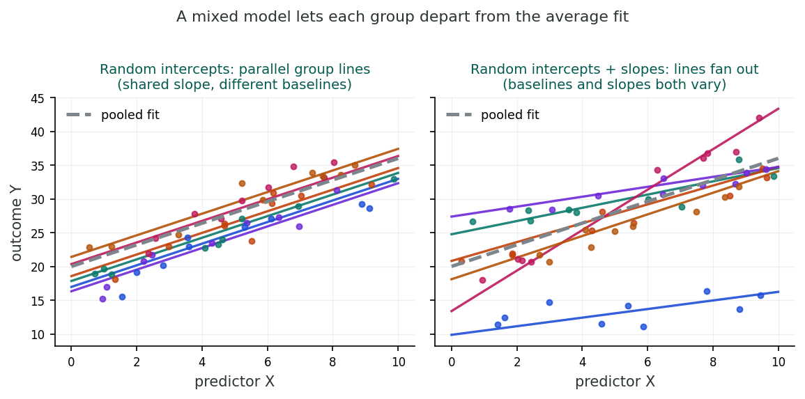
In plain terms, a random intercept lets each clinic’s line sit higher or lower while every line keeps the same tilt, so the fitted lines stay parallel. A random slope lets the tilt itself change from clinic to clinic, so a predictor can matter more in some clinics than in others. Picture a stack of parallel lines that you are now allowed to rotate one at a time: some steepen, some flatten, and a few may even swing the other way.
Random Intercept Model
In the random intercept model, all groups share the same slope for each predictor but have different baseline levels. The regression lines for different groups are parallel, shifted up or down by their random intercept. This is appropriate when you believe the effect of a predictor is consistent across groups but groups differ in their overall level of the outcome.
Random Intercept + Random Slope Model
In this extended model, each group can have both a different intercept and a different slope. The regression lines are no longer parallel: they can fan out, converge, or cross. This model requires estimating additional parameters: the variance of the random slope (σ²u1) and the covariance between the random intercept and slope (σu01). It is more flexible but also more complex and requires sufficient data.
The Covariance Matrix of Random Effects
When a model includes both random intercepts and random slopes, the random effects for each group are typically assumed to follow a bivariate normal distribution. The covariance matrix of the random effects includes three parameters: the variance of the random intercept (σ²u0), the variance of the random slope (σ²u1), and the covariance between them (σu01).
A positive covariance means groups with higher intercepts tend to have steeper slopes; a negative covariance means the opposite. This covariance should generally be estimated rather than assumed to be zero.
Hierarchical Model Interpretation
Random slopes models are sometimes called hierarchical or multilevel models because predictors can have effects at each level of the hierarchy. At the individual level, predictors explain variation within groups; at the group level, predictors or random effects explain variation between groups. This formulation shows that each predictor can enter as a fixed effect, a random effect at the group level, or both.
Imagine a multi-center clinical trial measuring blood pressure reduction across 30 hospitals. A random intercept model would allow hospitals to differ in their patients’ baseline blood pressure. A random slopes model would additionally allow the treatment effect itself to vary across hospitals, since some hospitals might show a larger treatment effect than others due to differences in patient populations, adherence, or clinical practice. The variance of the random slope tells you how much the treatment effect varies across sites.
Practical Considerations
Models with multiple random effects can have many parameters in the covariance matrix, and identifiability can become an issue. Practical parsimony is important: only include random effects for which there is theoretical justification and sufficient data. Adding unnecessary random effects can lead to convergence problems, unstable estimates, or singular covariance matrices.
1. A random slopes model allows:
2. In a random slopes model, the covariance between random intercept and slope:
3. Random slope models are sometimes called hierarchical models because:
Reflection
Consider a multi-center clinical trial where the treatment effect might vary across centers. What would a random slopes model for the treatment effect tell you that a random intercept model would not?
Contextual Effects & Statistical Analysis
Introduction and Overview
Within, between, and the gap between them. Once we let intercepts and slopes vary across clusters, a subtler issue surfaces: the same predictor can have a different effect depending on whether you look at variation within clusters or between them. Income predicts health one way at the individual level and another way at the neighbourhood level, and conflating the two is a common source of misleading conclusions. This section formalises that distinction (contextual effects), then turns to the statistical machinery for fitting and comparing mixed models: REML vs ML, likelihood-ratio tests for variance components, and the practical decisions that go with them. These ideas extend almost verbatim into later lessons.
Learning Objectives
- Define contextual effects and explain how within-group and between-group slopes can diverge.
- Apply group-mean centering to separate within-cluster from between-cluster effects.
- Distinguish ML from REML estimation and choose appropriately for fixed-effect vs variance-component inference.
- Use likelihood-ratio tests, including boundary corrections, to compare nested mixed models.
- Recognise the ecological and atomistic fallacies that follow from ignoring the contextual distinction.
Contextual Effects
A contextual effect occurs when a predictor measured at the individual level has a different effect depending on whether you examine variation within groups or between groups (Curran & Bauer, 2011). For a contextual effect to exist, two conditions must hold: (1) the predictor must vary both between and within groups, and (2) the within-group and between-group slopes must differ.
Understanding Contextual Effects
Imagine studying the relationship between income and health across neighborhoods. At the individual level (within a neighborhood), higher income might improve health modestly. But the neighborhood-level (between-group) effect of average income could be much stronger because wealthier neighborhoods have better infrastructure, cleaner environments, and more health services. The difference between these two slopes is the contextual effect: the additional benefit of living in a high-income neighborhood beyond one’s own income level.
Group-Mean Centering
To separate within-group and between-group effects, we can use group-mean centering. This replaces the original predictor X1i with:
The centered variable Z1i captures purely within-group variation (how an individual differs from their group mean). The group mean X1,group can then be included as a separate predictor to capture between-group variation.
Here, βW is the within-group effect and βB is the between-group effect. If βW ≠ βB, a contextual effect is present. Ignoring this distinction can lead to the ecological fallacy (wrongly attributing group-level associations to individuals) or the atomistic fallacy (wrongly attributing individual-level associations to groups).
Estimation Methods: ML vs. REML
Maximum Likelihood (ML)
ML estimation simultaneously estimates all parameters (fixed effects and variance components) by maximizing the full likelihood. However, ML does not account for the degrees of freedom used in estimating fixed effects, which leads to downward-biased estimates of variance components, analogous to dividing by n instead of n−1 in sample variance estimation (Patterson & Thompson, 1971). ML is required when comparing models with different fixed effects structures (e.g., likelihood ratio tests for fixed effects).
Restricted Maximum Likelihood (REML)
REML estimation adjusts for the degrees of freedom lost in estimating fixed effects by restricting the likelihood to a subspace orthogonal to the fixed effects (Patterson & Thompson, 1971). This produces less biased variance component estimates, especially when the number of groups is small. REML is generally the preferred method for estimating variance components. However, REML log-likelihoods are not comparable across models with different fixed effects.
Inference in Mixed Models
Wald tests are commonly used to test individual fixed effects. These are approximate tests that rely on asymptotic theory. For finite samples, approximations such as the Satterthwaite or Kenward–Roger methods provide better reference distributions (t or F) by estimating effective degrees of freedom (Kenward & Roger, 1997). These corrections are especially important when the number of groups is small.
To test whether a variance component is significantly different from zero (e.g., H0: σ²g = 0), we use a likelihood ratio test comparing the model with and without that random effect. However, because the null value (0) is on the boundary of the parameter space, the standard χ² reference distribution is too conservative. The recommended correction is to halve the P-value from the χ² test.
When comparing models with different random effects but the same fixed effects, use REML-based likelihood ratio tests (with P-value halving for boundary tests). When comparing models with different fixed effects, use ML-based likelihood ratio tests or information criteria (AIC, BIC). Always ensure that models being compared are nested and fit to the same data.
1. A contextual effect exists when:
2. REML estimation is generally preferred over ML because:
3. When testing whether a random effect variance is significantly different from zero:
Reflection
Explain in your own words why the ecological fallacy can occur when contextual effects are ignored. Give an example from epidemiology where the group-level and individual-level associations might differ.
Prediction, Residuals & Diagnostics
Introduction and Overview
From estimation to validation. Earlier sections walked through specifying, fitting, and interpreting linear mixed models. This final section addresses the questions that follow: how do we predict outcomes for individuals (with and without their cluster-specific deviation), what do BLUPs tell us about the clusters themselves, and how do we know whether the model fits? Mixed models have two layers of residuals, level-1 (within-cluster) and level-2 (between-cluster), and validating both is essential before drawing inferential conclusions. The diagnostic logic you build here transfers directly to the discrete-outcome and repeated-measures extensions in later lessons.
Learning Objectives
- Compute and interpret BLUPs (empirical Bayes estimates) of cluster-level random effects.
- Explain the shrinkage factor and why small clusters are pulled more strongly toward the overall mean.
- Distinguish level-1 (within-cluster) from level-2 (between-cluster) residuals and use both for diagnostics.
- Apply Box-Cox or alternative transformations to address non-normality of continuous outcomes in mixed models.
- Validate a fitted mixed model before reporting fixed-effect inferences.
BLUPs: Best Linear Unbiased Predictors
In a mixed model, the random effects u are not directly observed: they are latent variables. We estimate them using BLUPs (Best Linear Unbiased Predictors), which are the predicted values of the random effects conditional on the observed data (Laird & Ware, 1982; Bates et al., 2015).
The Shrinkage Factor
BLUPs are weighted averages of the group-specific estimate and the overall mean. The amount of shrinkage depends on the group size and the ICC:
When m (the group size) is large, the shrinkage factor approaches 1 and the BLUP closely approximates the raw group mean. When m is small, the factor is closer to 0 and the BLUP is pulled substantially toward the overall mean.
Partial pooling: the middle ground
Shrinkage is easiest to picture as a compromise between two extremes. One extreme is no pooling, where every cluster is fitted on its own data alone, so a three-patient clinic’s noisy average is trusted completely. The other extreme is complete pooling, where the clusters are ignored and a single line is fitted to everyone, as if the clinics were identical. A mixed model does neither. It applies partial pooling: each cluster’s estimate is a weighted blend of its own mean and the overall mean, and the weight is the shrinkage factor above. Data-rich clusters stay close to their own mean, while data-poor clusters lean on the crowd, which is what borrowing strength means in practice.
Consider a random intercept model for patient outcomes across hospitals. Suppose σ²g = 5 and σ² = 20. For a hospital with 100 patients: shrinkage factor = 5/(5 + 20/100) = 5/5.2 = 0.96, so the BLUP is very close to the hospital’s raw mean. For a hospital with only 4 patients: shrinkage factor = 5/(5 + 20/4) = 5/10 = 0.50, so the BLUP is pulled halfway toward the overall mean. This borrowing of strength from other groups is a key advantage of mixed models.
Residuals in Mixed Models
Mixed models produce multiple sets of residuals, one for each level of the hierarchy:
- Individual-level residuals (ε): the difference between observed values and the group-specific predictions (using BLUPs)
- Group-level residuals (u): the BLUPs themselves, representing how each group deviates from the overall mean
Model Diagnostics
Checking model assumptions in mixed models involves examining residuals at each level of the hierarchy. Variance explained at each level can also be summarised using marginal and conditional R² statistics (Nakagawa & Schielzeth, 2013). A recommended strategy is to work from the highest hierarchical level downward:
Practical Diagnostic Advice
Start by examining group-level residuals (BLUPs): check for normality using Q-Q plots and look for influential groups. Then examine individual-level residuals: check normality, homoscedasticity, and look for outliers. Working top-down helps identify whether problems originate at the group level rather than being caused by a few individual outliers within groups. Also check that residuals at each level are uncorrelated with predictors and fitted values.
Box-Cox Transformation for Mixed Models
When model assumptions (normality, homoscedasticity) are violated, a Box-Cox transformation of the response variable may help. In mixed models, the procedure involves computing transformed Y values for a range of λ values, fitting the same model to each, and comparing log-likelihoods. Crucially, ML estimation (not REML) must be used for comparing log-likelihoods across different λ values, because REML likelihoods are not comparable when the response variable changes.
1. BLUPs (Best Linear Unbiased Predictors) exhibit shrinkage, meaning:
2. When checking residuals in a mixed model, it is recommended to:
3. The Box-Cox transformation in mixed models:
Reflection
A random intercept model for hospital costs has a group of 5 hospitals with only 3 patients each and another group of 20 hospitals with 100 patients each. How would shrinkage affect the BLUP estimates differently for these two groups?
Lesson 10: Comprehensive Assessment
Bringing It All Together
This lesson built linear mixed models from the ground up (Laird & Ware, 1982; Bates et al., 2015). We started with the simplest specification, a random intercept that lets each cluster sit at its own baseline level, and used it to motivate the partition of total variance into between- and within-cluster components, summarised in the intraclass correlation coefficient. From there we relaxed the assumption that covariate effects are constant across clusters by introducing random slopes, hierarchical models, and cross-level interactions, and we examined the covariance structure that links random intercepts to random slopes.
The middle of the lesson confronted a subtler problem: even when a model is correctly specified mechanically, the same predictor can carry a different effect within clusters than between them. Group-mean centering separates those two effects cleanly, and the contextual-effects framework lets you avoid both ecological and atomistic fallacies. We then turned to the inferential machinery you actually use at the keyboard: REML versus ML estimation, likelihood-ratio tests for variance components (with the boundary correction they require), and the practical decisions about which random terms to keep.
The final section moved from estimation to validation: BLUPs as empirical-Bayes predictions of cluster-level random effects, the shrinkage factor that pulls small clusters toward the overall mean, two-level residual diagnostics, and Box-Cox transformations when the normality assumption is strained. These tools are the foundation for the next two lessons, where mixed models are extended to discrete outcomes (a later lesson) and to repeated-measures designs (a later lesson).
Key Takeaways from this lesson
- A linear mixed model partitions total variance into between-cluster (σ²g) and within-cluster (σ²) components; the ICC summarises how much of the variation lives between clusters.
- Random intercepts give each cluster its own baseline; random slopes additionally let predictor effects vary across clusters, with the random-effect covariance matrix capturing how intercepts and slopes co-vary.
- Within-group and between-group effects of the same predictor can differ; group-mean centering separates them and prevents the ecological and atomistic fallacies.
- REML is preferred for variance-component estimation; ML is required when comparing models that differ in fixed effects. Likelihood-ratio tests for variance components require a boundary correction.
- BLUPs (empirical Bayes predictors) of cluster random effects exhibit shrinkage toward the overall mean, more so for small clusters and lower ICCs.
- Mixed-model diagnostics operate on two levels of residuals; both must be examined before fixed-effect inferences are trusted.
This final assessment covers all material from this lesson. You must answer all 15 questions correctly (100%) and complete the final reflection to finish the lesson.
Reflection
Reflecting on this lesson, summarize the key decisions a researcher must make when fitting a linear mixed model (choosing fixed vs. random effects, estimation method, model diagnostics). Which aspect do you find most challenging?
Final Knowledge Assessment
1. In a linear mixed model, random effects are assumed to follow:
2. The variance component σ²g in a random intercept model represents:
3. If σ²g = 3 and σ² = 12, the ICC is:
4. A random slopes model differs from a random intercept model by:
5. The covariance between random intercepts and slopes in a random slopes model:
6. A contextual effect is detected when:
7. Group-mean centering replaces X1i with:
8. REML differs from ML estimation in that REML:
9. When comparing ML and REML for model selection:
10. Wald tests in mixed models:
11. BLUPs are also known as:
12. Shrinkage in BLUPs is stronger when:
13. Mixed models have residuals:
14. The Box-Cox transformation for mixed models requires using ML rather than REML because:
15. In a hierarchical model formulation, each predictor can enter the model:
✦ Before submitting: pass every section knowledge check (100%) and complete every reflection.