Crude OR
2.61
Fundamental Epidemiological Concepts and Approaches
This course was developed by Dr. Kiffer G. Card, Faculty of Health Sciences, Simon Fraser University based on Dohoo, I. R., Martin, S. W., & Stryhn, H. (2012). Methods in Epidemiologic Research. VER Inc.
📚 Reference page, available throughout the lesson
This glossary collects the key concepts, people, and ideas you will meet in this lesson. Use it as a reference while you work through the material, or as a review before assessments. Type in the search box to filter entries.
An earlier lesson closed the second leg of the bias triad with validity in observational studies. This lesson takes the third, confounding, and pulls together the full causal inference framework. Confounding is the systematic distortion of an exposure–outcome association by a third variable that influences both. The four content sections walk through the topic in the order an investigator would actually approach it. This section covers strategies that prevent confounding before data analysis (restriction, matching). A later section turns to detecting confounding in observed data and stratified analysis (Mantel–Haenszel). A later section introduces the analytic alternatives: multivariable regression, instrumental variables, propensity scores. A later section closes with what to do about confounders you can't measure, and how to think structurally about the relationships among extraneous variables.
A central focus of epidemiological research is to identify factors that contribute to the occurrence of disease. Randomised controlled trials (RCTs) provide a probabilistic basis for balancing factors between groups. However, in observational studies we cannot randomly assign exposures, so confounding is always a concern.
Confounding can be described as the mixing together of the effects of 2 or more factors. When confounding is present, we might think we are measuring the association between an exposure and an outcome, but the observed measure also includes the effects of one or more extraneous factors. These extraneous factors that produce the bias are called confounders or confounding factors.
A quick example to fix the idea: people who carry a cigarette lighter have far higher lung-cancer rates, yet the lighter itself causes nothing. Smokers are the people who carry lighters, and smoking is what raises cancer risk, so smoking gets mixed into any comparison of lighter-carriers with non-carriers. Smoking is the confounder here. Once you compare lighter-carriers and non-carriers who smoke the same amount, the apparent lighter effect vanishes. That is what it means to control for a confounder.
A factor is a confounder if:
Population confounder: known or regularly reported to be a confounder in the target population, should be controlled regardless of sample data.
Sample confounder: appears to be a confounder in the study data but may not truly be one in the population. We should not control for it unless there is substantive evidence.
Investigating the relationship between Streptococcus pneumoniae (STREP) and childhood respiratory disease (CRD), with RSV (respiratory syncytial virus) as a potential confounder:
| STREP+ | STREP− | OR | |
|---|---|---|---|
| CRD+ | 240 | 40 | 3.3 (crude) |
| CRD− | 6260 | 3460 |
When stratified by RSV status, the stratum-specific ORs are both 2.0, while the crude OR is 3.3. The >30% difference indicates confounding by RSV is present. The stratum-specific OR of 2.0 is the best estimate of the causal association.
We can prevent and control confounding using three general procedures:
In a cohort study, matching makes the exposure independent of the matched extraneous variable so there can be no confounding. The matched variable(s) can still exert an effect on the outcome, but it has the same effect in both exposure groups.
Because the outcome (e.g., disease) has not happened at the time of matching, the matching process is independent of the outcome. No analytical control of the matched confounder is necessary, and there is no bias in the summary table.
In case-control studies, the disease has already occurred when matching takes place. Matching will actually introduce a selection bias. The stronger the exposure-confounder association, the greater the bias (generally toward the null).
This bias must be controlled by stratified or matched analysis; the matched variable(s) must be included in the analytical approach.
Do not match unless you are certain the variable is a confounder. Matching on a variable strongly associated with exposure but not a confounder leads to overmatching, giving the distribution of exposure in controls greater similarity to cases than in the source population, which can reduce precision.
| Feature | Frequency Matching | Pair Matching |
|---|---|---|
| Method | Overall distribution made equal | Individual-level matching (1:m) |
| Analysis | Stratified (MH procedure) | Matched-pair analysis (McNemar’s test) |
| Interaction | Can assess interaction | Difficult to assess interaction |
| Best when | Confounder has few levels | Many variables or refined categories |
| Control-to-case ratio | Variable | Fixed (1:1, 1:4, etc.); minimal gain beyond 4:1 |
For pair-matched data in a case-control study with 1:1 matching, we analyse the four possible exposure patterns. Only the discordant pairs (case exposed/control unexposed, or case unexposed/control exposed) contribute information:
where u = pairs where case is exposed and control is not, and v = pairs where case is not exposed and control is.
Why do the other pairs drop out? If a case and their matched control were both exposed (or both unexposed), the pair shows the same exposure on each side, so it says nothing about whether exposure differs between cases and controls. Only the discordant pairs, where exactly one of the two was exposed, carry that information.
Why does matching in case-control studies introduce selection bias while matching in cohort studies does not? Think about the timing of when disease occurs relative to the matching process.
Minimum 20 characters required.
1. Which of the following is not a criterion for a factor to be a confounder?
2. In a case-control study, matching on a confounder:
3. The McNemar’s test is used for:
An earlier section covered the strategies that prevent confounding before any data are looked at. This section takes over once the data are in: how do we tell whether a candidate variable is actually confounding the exposure–outcome relationship, and how do we adjust for it via stratification? Mantel–Haenszel is the workhorse method here and the conceptual ancestor of every multivariable regression you'll meet in a later course.
Identifying which potential confounders need to be controlled can be accomplished using directed acyclic graphs (DAGs) (Greenland, Pearl, & Robins, 1999). The process:
Watch the front door (causal) and back door (confounded) of a DAG, then close the backdoor by conditioning. Next ▶ advances scenes.
A 7-scene visualization of Pearl's backdoor criterion: nodes E, Y, and confounder C; the causal front door E→Y; the spurious backdoor through C; conditioning on C as the door slamming shut; and the ice-cream/drownings example to ground the abstraction.
In studying the effect of cigarette smoking (CIG) on birth weight (BWT), with RACE, COLLEGE, TBO (total birth order), and WTGAIN as additional factors:
A practical approach: compare the crude OR (ORc) with the adjusted OR (ORa) obtained after stratification. If the change exceeds 20–30%, confounding is considered important.
The odds ratio is not always collapsible: even in the absence of confounding, the crude OR can differ from the stratum-specific ORs (Greenland, Robins, & Pearl, 1999). This typically occurs when outcome frequency is high. A >20–30% change in OR might look like confounding but could simply be non-collapsibility.
In plain terms: the odds ratio does not blend across subgroups the way a risk ratio does, so merging strata can nudge it even when nothing is being confounded. When the outcome is common, treat a modest odds-ratio change after stratifying with extra caution, and consider checking the risk ratio, which does not have this quirk.
The Mantel-Haenszel (MH) procedure (Mantel & Haenszel, 1959) is the most widely used stratified analytic approach. It involves physically stratifying data by levels of the confounder(s), examining stratum-specific ORs, and computing a pooled ‘adjusted’ estimate.
A study with 2,000 participants. Adjust how strongly the confounder C is linked to the exposure and to the outcome, then watch the crude OR diverge from the stratum-specific ORs and the pooled ORMH. The change-in-estimate ("Δ") tells you whether stratification matters.
| Y+ | Y− | Total | |
|---|---|---|---|
| E+ | 281 | 536 | 817 |
| E− | 198 | 985 | 1183 |
| Y+ | Y− | |
|---|---|---|
| E+ | 239 | 278 |
| E− | 145 | 338 |
| Y+ | Y− | |
|---|---|---|
| E+ | 42 | 258 |
| E− | 53 | 647 |
Interaction occurs when the combined effect of 2 variables differs from the sum (or product) of their individual effects. There are 3 types of joint effects:
When stratum-specific measures differ significantly (interaction is present), we should not compute a single summary ORMH. Instead, we must report stratum-specific estimates because the effect of the exposure depends on the level of the other variable. This phenomenon is also called effect modification.
Consider a study where the crude OR is 1.69 and the Mantel-Haenszel adjusted OR is 1.97 (a 17% change). Would you consider this sufficient evidence of confounding? What factors would influence your decision?
Minimum 20 characters required.
1. In the Mantel-Haenszel procedure, before interpreting ORMH, you should first:
2. Non-collapsibility of the odds ratio means that:
3. In the context of interaction, if RR10 × RR01 ≠ RR11, this indicates interaction on the:
Stratification works beautifully for one or two confounders but breaks down quickly when you need to adjust for several at once. This section turns to the analytic methods that scale beyond a few strata: multivariable regression (the workhorse of a later course), and the alternatives of restriction-by-design, instrumental variables, and propensity scores. Each is a different strategy for the same goal of estimating the exposure–outcome effect while making the remaining differences between groups irrelevant.
The most commonly used analytical method for controlling confounding is to include confounders in a multivariable model (e.g., logistic regression). The effect of the exposure is estimated while holding other factors constant.
If the coefficient for a predictor changes by >30% when a putative confounder is added to the model, then substantial confounding exists. Note that the ‘adjusted’ measures from multivariable models are direct causal effects only, not total causal effects.
Standardisation uses stratum-specific risks applied to a standard population. The SRR compares observed vs. expected number of cases:
Unlike the MH estimator, the SRR provides a valid summary even in the presence of interaction, because the population of interest is specified. The SRR is a non-parametric method based on physical stratification.
The marginal structural model (Robins, Hernán, & Brumback, 2000) uses weights to create an unconfounded pseudo-population from which the causal effect can be estimated using a crude (marginal) measure.
The weight assigned to each subject is the inverse probability of treatment weight (IPTW): WT = 1/pE, where pE = p(E=e|C) is the conditional probability of the observed exposure given confounders.
The total pseudo-population is twice the size of the observed population and contains information on the counterfactual outcome. The IPTW estimate is equivalent to the SRRtot estimate.
An instrumental variable (IV) Z (Angrist, Imbens, & Rubin, 1996; Hernán & Robins, 2006) must meet 3 requirements:
The true causal effect (TCE) is estimated as:
The key advantage: we do not need to condition on confounders C. The IV approach bypasses confounding entirely. However, finding a valid IV in observational studies is very difficult.
A propensity score (PS) is the conditional probability of being treated/exposed given measured covariates: p(E+|C). Propensity scores condense multiple confounders into a single scalar summary (Rosenbaum & Rubin, 1983; Austin, 2011).
With 1–2 categorical confounders, PSs can be calculated manually. With more confounders, use a logit or probit model predicting treatment (exposure) allocation as the outcome. Include all potential confounders (known or suspected) and their interactions.
A study is balanced if: (1) the average PS value is the same in exposed and non-exposed within each PS stratum, and (2) the mean of all covariates making up the PS is equal across groups within each stratum.
Analysis is limited to the region of common support, the observations falling in the range of PSs that includes both exposed and non-exposed individuals.
PSs can be used in four ways:
| Method | Description |
|---|---|
| Matching | Match exposed to non-exposed with similar PSs. Methods: nearest-neighbour, radius, kernel matching |
| Stratification | Divide into PS strata (blocks); compute att within each stratum and pool |
| Covariate in model | Include PS as a continuous or categorical variable in the regression model |
| Weighting (IPTW) | Weight observations by inverse of PS to create pseudo-population |
The most common effect measure with PS methods is the average treatment effect in the treated (att): the difference in outcome between treated (exposed) and non-treated (non-exposed) groups.
The companion R script r-activities/HSCI_341_Lesson_12_Confounding_and_Causal_Inference.R walks through two confounding-control workflows: (A) a Mantel-Haenszel adjusted OR for smoking and lung cancer stratified by age (with stratum-specific ORs to check for effect modification), and (B) an inverse-probability-of-treatment weighted (IPTW) logistic regression with a known simulated treatment effect of log-OR = 0.5.
# PART A -- Mantel-Haenszel adjusted OR (2x2x2 array)
arr <- array(c( 22, 5,    10, 25,
                75, 15,   35, 85),
              dim = c(2, 2, 2),
              dimnames = list(Smoke = c("Yes", "No"),
                              Case  = c("Yes", "No"),
                              Age   = c("Young", "Old")))

mantelhaen.test(arr, exact = FALSE)             # MH OR + CI
apply(arr, 3, function(t) (t[1,1]*t[2,2]) / (t[1,2]*t[2,1])) # stratum-specific

crude <- margin.table(arr, c(1, 2))             # collapse strata
(crude[1,1]*crude[2,2]) / (crude[1,2]*crude[2,1])    # crude OR

# PART B -- inverse-probability-of-treatment weighting
set.seed(341)
n   <- 2000
age <- rnorm(n, 60, 10)
A   <- rbinom(n, 1, plogis(-3 + 0.05*age))         # treatment
Y   <- rbinom(n, 1, plogis(-2 + 0.04*age + 0.5*A))  # outcome (true log-OR=0.5)
df  <- data.frame(age, A, Y)

ps_mod <- glm(A ~ age, data = df, family = binomial)
ps     <- predict(ps_mod, type = "response")
w      <- ifelse(df$A == 1, 1/ps, 1/(1-ps))         # IPTW

coef(glm(Y ~ A, data = df, family = binomial))["A"]                # crude
coef(glm(Y ~ A, data = df, family = binomial, weights = w))["A"]    # IPTW
What you should be able to do after this activity: compute and compare crude, stratum-specific, and Mantel-Haenszel ORs; estimate a propensity score; build IPT weights; and check whether the weighted estimate recovers a known simulated effect.
Use the questions below to interpret the actual numbers from your Mantel-Haenszel and IPTW outputs. Look at the console before answering.
1. From mantelhaen.test(arr, exact = FALSE), report the common (adjusted) OR with its 95% CI. How does it compare to the crude OR you computed from margin.table()? What does the difference (or lack of difference) say about age as a confounder?
mantelhaen.test(arr, exact = FALSE) returns a common (adjusted) OR of about 11.9, with a 95% CI comfortably above 1, so the smoking and lung cancer association is strong and clearly non-null. The crude OR from margin.table() is almost identical, also about 11.9, because (97×110)/(45×20) = 11.9. Since the adjusted and crude estimates barely differ, far below the usual change-in-estimate threshold, age is NOT confounding these data: stratifying on age leaves the odds ratio essentially unchanged. A variable earns the label confounder only when adjusting for it actually moves the estimate.2. The apply() line printed two stratum-specific ORs (Young, Old). Report both. Are they similar enough to justify a single MH summary OR, or is there evidence of effect modification (i.e., the OR differs substantially by stratum)?
apply() line returns stratum-specific ORs of about 11.0 for the Young stratum, since (22×25)/(10×5) = 11.0, and about 12.1 for the Old stratum, since (75×85)/(35×15) = 12.1. They sit close to one another and to the pooled MH value of about 11.9, so the odds ratios are homogeneous and a single Mantel-Haenszel summary is justified. Effect modification would instead show strata that differ substantially, for example an OR near 3 in one stratum and near 15 in the other; a formal Breslow-Day or Tarone homogeneity test would not reject homogeneity here.3. Compare the crude coef(...)["A"] and the IPTW-weighted coef(..., weights = w)["A"]. Which is closer to the true simulated log-OR of 0.5, and why would the IPTW estimate be biased if you had OMITTED age from ps_mod?
ps_mod, the propensity score would not adjust for the confounding age induces, so the IPTW estimate would inherit the same age-driven bias as the crude analysis, drifting back toward 0.66. The general lesson: propensity-score methods depend critically on the no-unmeasured-confounders assumption; omitting a confounder from the PS model defeats the purpose of using PS at all.Compare the propensity score approach to traditional multivariable regression for controlling confounding. In what situations might propensity scores be preferable, and what are their limitations?
Minimum 20 characters required.
1. A propensity score is best described as:
2. An instrumental variable must satisfy all of the following except:
3. The “region of common support” in propensity score analysis refers to:
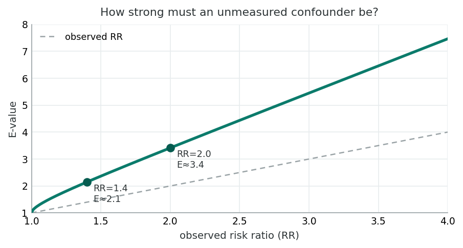
The E-value is the minimum strength of association that an unmeasured confounder would need with both exposure and outcome to fully explain the observed effect. Larger E-values indicate more robust findings. The formula shown applies when RR > 1; analogous forms exist for the OR and hazard ratio.
Earlier sections covered the methods that work when confounders are measured. This section tackles the harder case: what to do when key confounders are unmeasured or unknown. Sensitivity analyses, E-values, and structural reasoning about extraneous variables (mediators, colliders, effect modifiers) all give the working investigator tools for stating, transparently, how robust their conclusions are to the confounders they could not adjust for.
When a confounder was not measured in the study but information about its distribution exists from external sources, we can estimate what the adjusted measure would have been using external adjustment. The method works by estimating the cell values that would be expected if the confounder had been measured.
Click to explore how external data on RSV prevalence can be used to estimate adjusted OR when RSV was not directly measured in the study.
In our STREP-CRD study, suppose RSV status was not measured. From external data we know:
Using the crude data (a = 70, b = 30, c = 90, d = 210):
| Stratum | a | b | c | d |
|---|---|---|---|---|
| RSV+ (estimated) | 28 | 3 | 42 | 27 |
| RSV− (estimated) | 42 | 27 | 48 | 183 |
The MH OR from these estimated strata approximates the adjusted OR, illustrating how external information can help address unmeasured confounding, though with important assumptions about the accuracy of the external prevalence data.
When no external data are available, sensitivity analysis explores how strong an unmeasured confounder would need to be to explain away an observed association. This does not eliminate confounding but quantifies the threat it poses to the study’s conclusions.
Click to see how varying assumptions about an unmeasured confounder’s strength affects the adjusted estimate.
Suppose we observe a crude OR = 5.44 for the STREP-CRD association. We suspect an unmeasured confounder Z might exist.
We systematically vary two parameters:
| ORZD | p1=0.4, p2=0.1 | p1=0.6, p2=0.1 | p1=0.8, p2=0.1 |
|---|---|---|---|
| 2.0 | 4.68 | 4.07 | 3.44 |
| 5.0 | 3.51 | 2.50 | 1.64 |
| 10.0 | 2.67 | 1.63 | 0.91 |
Even with a moderately strong unmeasured confounder (ORZD = 5, prevalence difference of 30%), the adjusted OR remains above 2.5, suggesting the STREP-CRD association is reasonably robust to unmeasured confounding.
Think about a published observational study you have encountered (or one from class). What unmeasured confounders might threaten its conclusions? How could sensitivity analysis help evaluate the robustness of its findings?
The relationship between exposure (E), disease (D), and an extraneous variable (F) can take many forms. Understanding these patterns is critical for correctly interpreting what happens when you “control for” a variable.
Click to reveal
F → D (no E-F link)
F causes D independently of E. Controlling for F does not change the E-D measure. There is an F-D association but no E-F association. F is not a confounder.
Click to reveal
F → E → D
F causes E, which causes D. Controlling for F does not change the E-D measure. There is an F-D association and an E-F association. F is not a confounder; it acts through E.
Click to reveal
F → E and F → D (no E→D)
F causes both E and D, but E does not cause D. Controlling for F eliminates the E-D association. This is complete confounding: the entire observed E-D link is spurious.
Click to reveal
F → E and F → D and E → D
F causes both E and D, but E also independently causes D. Controlling for F changes but does not eliminate the E-D association. This is partial confounding, the classic confounder scenario.
Click to reveal
E → F → D
E causes F, which causes D (F is on the causal pathway). Controlling for F reduces or eliminates the E-D association. F should generally not be controlled for, as it would mask E’s true effect.
Click to reveal
F distorts a null E-D relationship
There is no true E-D association, but F creates a spurious one. Crude analysis shows E-D association; controlling for F reveals the null. Both F-D and E-F associations exist. A distorter is a confounder that creates a false positive.
Click to reveal
F suppresses a true E-D relationship
A true E-D association exists but is hidden in crude analysis because F masks it. Controlling for F reveals or strengthens the E-D association. A suppressor is a confounder that creates a false negative.
Click to reveal
F modifies the E → D effect
F changes the magnitude of the E-D association across its strata. Controlling for F reveals different stratum-specific measures. Effect modification is a biological phenomenon, not a bias, so stratum-specific results should be reported separately.
| Type | E-D changes? | F-D assoc? | E-F assoc? | Confounder? |
|---|---|---|---|---|
| Exposure-independent | No | Yes | No | No |
| Simple antecedent | No | Yes | Yes | No |
| Explanatory (complete) | Yes → null | Yes | Yes | Yes |
| Explanatory (incomplete) | Yes → attenuated | Yes | Yes | Yes |
| Intervening variable | Yes → reduced | Yes | Yes | No* |
| Distorter | Yes → null | Yes | Yes | Yes |
| Suppressor | Yes → stronger | Yes | Yes | Yes |
| Moderator | Varies by stratum | May vary | May vary | No** |
*Controlling for an intervening variable is usually inappropriate.
**Effect modification is a biological phenomenon, not bias.
Confounding is a fundamental threat to causal inference in observational studies. Its control requires a combination of study design strategies (restriction, matching) and analytical approaches (stratification, multivariable modelling, propensity scores). The choice among methods depends on the research question, data structure, and assumptions the investigator is willing to make.
Click to review how different methods yielded similar adjusted estimates.
| Method | OR Estimate | Key Feature |
|---|---|---|
| Crude (unadjusted) | 5.44 | No control for RSV |
| Restriction (RSV− only) | 3.21 | Limits generalizability |
| MH Stratification | 3.38 | Transparent, stratum-specific |
| Mantel-Haenszel (pooled) | 3.38 | Weighted average across strata |
| Logistic Regression | 3.40 | Handles multiple confounders |
| Propensity Score | ~3.4 | Balances many covariates |
| External Adjustment | ~3.4 | Uses external prevalence data |
All methods converge on a similar adjusted OR of approximately 3.4, down from the crude OR of 5.44. This consistency strengthens confidence that RSV confounds the STREP-CRD association and that the true effect of STREP on CRD is approximately 3-fold.
Question 1: In sensitivity analysis for unmeasured confounding, what is the primary goal?
Question 2: A researcher finds that controlling for variable F completely eliminates the association between exposure E and disease D. F is associated with both E and D. Which type of extraneous variable is F most likely?
Question 3: Why should an intervening (mediating) variable generally not be controlled for in analysis?
Consider a real-world observational study (e.g., the association between coffee consumption and heart disease). Identify at least one potential unmeasured confounder and describe how you would design a sensitivity analysis to evaluate its impact on the study conclusions.
Minimum 20 characters required.
This lesson closed the third leg of the bias triad and pulled together the full causal-inference framework for observational research. The arc moved from design-stage confounding control (restriction, matching), through detection and stratified analysis (DAGs, change-in-estimate, Mantel-Haenszel), into the analytic methods that scale (multivariable regression, marginal structural models, instrumental variables, propensity scores), and finally to the harder problem of confounders that are unmeasured or unknown (external adjustment, sensitivity analysis, E-values, the eight types of extraneous variables).
The final assessment below asks you to integrate across all four sections: identifying confounders by their three criteria, choosing among design and analytic strategies, computing and interpreting Mantel-Haenszel and propensity-score estimates, and articulating what an observational study can and cannot say about causation. The recurring example, STREP and childhood respiratory disease, with RSV as the confounder, runs through every method to make the abstractions concrete.
This lesson is the capstone of this course's analytic arc. What you take away here is what the regression and modelling lessons of a later course, Exploratory Data Analysis for Epidemiology (logistic regression, mixed models, survival analysis) build on: every adjusted estimate in that course is a confounding-control claim, and the tools you have just learned are how you decide whether the claim is defensible. For the modern target-trial framing of observational causal inference see Hernán & Robins (2016).
An earlier section: Definition of confounding and the three criteria for a confounder, population vs. sample-level confounding, pre-analysis control through restriction and matching (frequency and pair matching), McNemar’s test for matched pairs (Eqs 12.2–12.3), and the risk of overmatching.
An earlier section: Detection of confounding via DAGs and the change-in-estimate approach (20–30% threshold), non-collapsibility of the odds ratio, Mantel-Haenszel stratified analysis (Eqs 12.4–12.9), interaction and effect modification (additive vs. multiplicative), and when to report stratum-specific results.
An earlier section: Multivariable modelling and the 30% change rule for variable inclusion, standardisation and marginal structural models, instrumental variable analysis and the exclusion restriction, propensity score methods (matching, stratification, weighting, covariate adjustment), and the region of common support.
An earlier section: External adjustment for unmeasured confounders using external prevalence data (Eq 12.12), sensitivity analysis to quantify the threat of unmeasured confounding, eight types of extraneous variable relationships (exposure-independent, simple antecedent, explanatory antecedent with complete/incomplete confounding, intervening variable, distorter, suppressor, moderator), and comparison of confounding control methods.
The final reflection below asks you to apply sensitivity reasoning to a real-world question. The 15-question assessment that follows it covers all material from earlier sections. You must answer every question correctly to complete the lesson.
Pick one observational study you have read this term whose conclusions hinge on confounding control (your own capstone, the STREP-CRD example, or a published study you appraised). Identify a confounder you would worry was unmeasured, sketch how you would conduct a sensitivity analysis or compute an E-value to bound its possible impact, and state what you would conclude about the study's claim if your analysis showed the result was robust, or fragile, to that confounder.
Minimum 20 characters required.
Question 1: Which of the following is not one of the three criteria for a variable to be a confounder?
Question 2: In a case-control study using frequency matching, what is the primary purpose?
Question 3: What is “overmatching” in the context of confounding control?
Question 4: A DAG shows arrows from F to E and from F to D, with no arrow from E to D. What does controlling for F reveal?
Question 5: The change-in-estimate approach typically considers confounding present when the crude and adjusted measures differ by more than:
Question 6: In the Mantel-Haenszel method, the ORMH is calculated as:
Question 7: What distinguishes effect modification from confounding?
Question 8: Which confounding control method balances many covariates simultaneously using a single composite score?
Question 9: In a cohort study, restriction as a confounding control method involves:
Question 10: What is the “region of common support” in propensity score analysis?
Question 11: A “suppressor” variable is one that:
Question 12: Why is non-collapsibility a concern when using the odds ratio?
Question 13: An instrumental variable (IV) must satisfy which key condition?
Question 14: Sensitivity analysis for unmeasured confounding helps researchers by:
Question 15: Which statement about confounders at the population level versus the study sample level is correct?