Controlled
Studies
Fundamental Epidemiological Concepts and Approaches
Learning objectives for this lesson:
- Design a controlled trial that produces a valid and efficient evaluation of an intervention
- State trial objectives clearly and specify the target and source populations
- Describe the phases of clinical research from Phase 0 through Phase IV
- Allocate subjects to interventions using simple, stratified, cross-over, factorial, cluster, and split-plot randomisation
- Distinguish single, double, and triple blinding and identify the bias each prevents
- Compute and interpret sample size requirements, including the inflation factor for cluster randomised trials
- Compare intent-to-treat and per-protocol analyses and identify when each is appropriate
- Define direct, indirect, and total vaccine efficacy and apply the equations to a worked example
- Apply the CONSORT 2010 reporting standards to plan and report a randomised trial
This course was developed by Dr. Kiffer G. Card, Faculty of Health Sciences, Simon Fraser University based on Dohoo, I. R., Martin, S. W., & Stryhn, H. (2012). Methods in Epidemiologic Research. VER Inc.
Glossary: Key Terms, People & Concepts
📚 Reference page, available throughout the lesson
This glossary collects the key concepts, people, and ideas you will meet in this lesson. Use it as a reference while you work through the material, or as a review before assessments. Type in the search box to filter entries.
Foundations of RCTs & Trial Setup
⏱ Estimated reading time: 18 minutes
What makes a trial randomised
A randomised controlled trial allocates participants to interventions using a formal chance-based mechanism, then follows them for outcomes.
Random allocation produces baseline comparability on both measured and unmeasured factors. That is the property no observational design can match.

Introduction and Overview
Earlier lessons worked through the observational designs, including cross-sectional, cohort, case-control, ecological, and the hybrid variants. Every one of them measures exposure as it occurs naturally, and every one of them must spend effort defending against confounding. This lesson turns to the experimental alternative: when the investigator controls who is exposed via random assignment, confounding is broken by the design itself rather than by statistical adjustment. The three content sections move through an RCT in the order an investigator would build one: foundations and setup (this section), the central design choices around allocation, outcome measurement, sample size, and blinding (a later section), and finally the conduct, analysis, and reporting of the trial (a later section).
Learning Objectives
- Define a randomised controlled trial and explain why RCTs are considered the gold standard for evaluating interventions.
- Describe the five phases of clinical research from pre-clinical work through Phase IV post-marketing surveillance.
- Distinguish between target population, source population, and study group.
- Develop appropriate eligibility criteria that balance internal validity with generalisability.
- Specify an intervention with the precision needed for replication.
What Is a Randomised Controlled Trial?
A randomised controlled trial (RCT) is a planned experiment in which the investigator deliberately allocates participants to one or more interventions, then follows them to observe outcomes. Because the allocation is determined by the investigator (rather than by self-selection or by clinical circumstance), randomisation produces groups that are comparable on both measured and unmeasured factors at baseline. This is the property that gives the RCT its inferential power.
Walk through the first modern RCT, the trial that turned scarcity into science. Next ▶ advances scenes.
A 7-scene retelling of the 1948 MRC streptomycin trial: postwar TB epidemic, the scarce U.S. drug shipment, Bradford Hill's elegant solution (random allocation), the slot-machine randomization, dramatic 6-month outcomes, BMJ publication, and the rise of the RCT as gold standard.
Throughout this lesson we follow the chapter convention of using RCT to describe any planned experiment evaluating products or procedures outside the laboratory. The terms clinical trial (often restricted to therapeutic products in clinical settings) and field trial (carried out in general population settings) are used interchangeably with RCT. The factor under investigation is called the intervention; the effect of interest is called the outcome; people or groups participating are called subjects or participants. The lineage of the controlled comparison reaches back to James Lind's 1753 shipboard trial of citrus for scurvy, but it was the 1948 MRC streptomycin trial that introduced formal random allocation as the design's defining feature.
Why RCTs Are the Gold Standard
RCTs allow much better control of potential confounders than observational studies and reduce bias from selection and misinformation. By randomly assigning the intervention, the investigator breaks any link between exposure and unmeasured confounders, a feat that no observational design can match. As Lavori and Kelsey put it, the RCT is at present the unchallenged source of the highest standard of evidence used to guide clinical decision-making. That said, a single RCT is rarely sufficient to answer questions about complex interventions, and concerns persist that some trials lack relevance to real-world practice.
CONSORT and Trial Registration
The Consolidated Standards of Reporting Trials (CONSORT) statement was developed to improve the quality of trial reporting. It was first published in 1996, updated in 2001, and again in 2010 (Schulz, Altman, & Moher, 2010). We will use its main headings as the structural template throughout this lesson; the full 25-item checklist appears in a later section. As of 2005, the International Committee of Medical Journal Editors required investigators to register their trials prior to participant enrolment as a precondition for publishing in member journals. The WHO operates an International Clinical Trials Registry Platform (ICTRP), although registration remains effectively voluntary in many jurisdictions.
The Phases of Clinical Research
While controlled trials are valuable for assessing a wide range of factors affecting health, one of their most common uses is to evaluate pharmacological products. Before any trial in humans, extensive pre-clinical studies are conducted in vitro (test tube or cell culture) and in vivo (animal) using wide-ranging doses to obtain preliminary efficacy, toxicity, and pharmacokinetic information.
Click any phase to see its purpose, typical sample size, and key design features.
First-in-Human
Safety
Efficacy Signal
Pivotal Efficacy
Post-Marketing
Background, Objectives, and Trial Design
The objectives of a trial must be stated clearly and succinctly. A good objective describes the intervention, the allocation design (parallel, factorial, cross-over, etc.), and the primary outcome(s). Each trial should have a limited number of objectives plus, if needed, a small number of secondary outcomes. Increasing the number of objectives complicates the protocol, jeopardises compliance, and sacrifices statistical power.
Most trials contrast two groups, intervention and comparison, and are sometimes referred to as two-arm studies. Trials with more arms can be efficient when factorial designs are used (a later section). The comparison group might receive a placebo, no treatment, the usual treatment, or a different dose of the same product.
Choosing the Comparator: A Consequential Decision
Placebos are ideal when there is no established alternative intervention; where possible, a placebo is preferred to “no treatment.” However, when an effective standard treatment exists, withholding it from the comparison arm may be unethical; randomisation is ethically defensible only when there is genuine uncertainty in the expert community about which arm is superior, a state Freedman (1987) called clinical equipoise. In these settings, the standard of care serves as the comparator, and the trial may take the form of a non-inferiority trial, which aims to show the new intervention is no worse than the existing standard by more than a clinically unimportant margin (delta). Determining the appropriate value of delta is one of the most consequential design decisions in a non-inferiority trial.
Example 12.1: A Trial of Prostate Cancer Screening
The Andriole and colleagues (2012) trial randomised 38,340 men aged 55–74 to a screening intervention and 38,345 to usual care across 10 USA screening centres between 1993 and 2001. Men in the intervention arm were offered annual PSA tests for six years and digital rectal examination for four years. Follow-up extended through 2009 or 13 years from trial entry. The primary analysis was an intention-to-screen comparison of prostate cancer-specific mortality. The trial illustrates how a clearly stated objective (mortality reduction from screening) can be embedded in a simple two-arm parallel design that can nonetheless run for two decades.
Notice that the comparator was “usual care,” which sometimes included opportunistic screening. This pragmatic choice (Tunis, Stryer, & Clancy, 2003; Loudon et al., 2015) makes the results applicable to the real US health system but complicates interpretation of the “true” effect of organised screening.
Participants: Defining the Study Group
Three nested populations must be distinguished in any trial:
Figure 12.1. The target population is the group to which results should generalise. The source population is the subset that is eligible and reachable. The study group is the smaller subset that meets eligibility criteria and consents to participate.
Defining the Three Populations
- Target population: the population to which you want results to apply. Stating this explicitly helps ensure that conclusions remain practical and relevant.
- Source population: representative of the target population and consisting of eligible subjects from whom the study group is drawn. The setting and location of the source population should be described.
- Study group: the actual subjects who fit inclusion/exclusion criteria and agree to participate. Volunteers are unavoidable; how well they represent the source and target populations must be considered when extrapolating results.
Unit of Concern: Individuals or Clusters?
An early decision is the level at which the intervention will be applied. Some interventions can only be delivered to groups (e.g., medication added to drinking water; a school-wide curriculum). When the intervention is applied at the group level and the outcome is measured at the group level, this is a group-level study. When the outcome is measured on individuals within those groups, this is a cluster randomised study, which is discussed in a later section.
Eligibility Criteria
Adequate records should be available to verify previous health history, prior treatments, and any condition relevant to the trial. This is especially important when the intervention may interact with prior therapies.
For trials of therapeutic agents, a precise definition of the disease being treated is essential. Subjects who do not actually have the condition will dilute any treatment effect and reduce statistical power.
For trials of preventive products, healthy subjects are required, and procedures must be in place to confirm and document health status at the start of the trial.
Restricting a trial to subjects most likely to benefit increases statistical power but may limit generalisability. Subjects at high risk for adverse effects should generally be excluded both for ethical reasons and to protect the validity of the safety assessment.
The Width of Eligibility Criteria: A Trade-off
A narrow set of eligibility criteria yields a more homogeneous response and increases statistical power, but reduces generalisability. A broad set increases the pool of potential participants and can reveal subgroup variation, but introduces greater background variability that may hurt overall power. The recommended balance: use criteria reflecting the breadth of subjects who would receive the intervention in real-world practice if it proves effective.
Specifying the Intervention
The nature of the intervention and how it is administered must be clearly defined, with enough detail that another investigator could replicate it. Interventions vary widely:
- Medical interventions (e.g., creatine supplementation, antibiotic regimens)
- Surgical techniques (e.g., single-layer vs. double-layer uterine closure)
- Devices or instruments (e.g., progressive lenses for presbyopia)
- Screening programmes (e.g., PSA testing for prostate cancer)
- Behavioural programmes (e.g., adolescent smoking cessation)
A fixed intervention (one with no flexibility) is appropriate for assessing new products in Phase III trials. A more flexible protocol is appropriate for products that have been in use long enough that some clinical judgment has accumulated. Whenever possible, the initial treatment assignment should remain masked so clinical decisions are not influenced by knowledge of group allocation. Clear instructions are critical when participants administer some or all of the intervention themselves (such as instructions for taking medication). A monitoring system should be in place to verify that the intervention is delivered as planned.
Example 12.2: A Sequential Trial of Creatine in ALS
Groeneveld and colleagues (2003) recruited ALS patients from neuromuscular outpatient clinics in Utrecht and Amsterdam. The two interventions were creatine monohydrate and a matching placebo, designated A and B. An independent physician, masked to assignment, instructed the research pharmacist which medication to dispense. Patients were seen at 1 month, 2 months, and every 4 months thereafter. Reasons for withdrawal (serious adverse events, withdrawal of consent) were documented; patients who stopped trial medication remained in the intent-to-treat analysis. The careful specification of this masking-and-allocation chain, from the masked physician through the pharmacist to the patient, illustrates how an unambiguous intervention specification protects the integrity of the trial.
Key Takeaways
- RCTs are the gold standard for evaluating interventions because random allocation breaks the link between exposure and unmeasured confounders.
- Clinical research progresses through pre-clinical studies, then Phase 0 (first-in-human), Phase I (safety), Phase II (efficacy signal), Phase III (pivotal efficacy), and Phase IV (post-marketing surveillance).
- The CONSORT 2010 statement structures both trial design and reporting; trial registration is required by major journals.
- Three nested populations matter: the target population (who results should apply to), the source population (eligible and reachable), and the study group (eligible + consenting).
- Eligibility criteria balance internal validity against generalisability. Recommend using criteria that mirror who would receive the intervention in real practice.
- Interventions must be specified with the precision needed for replication, and a monitoring system should verify delivery.
1. Phase II clinical trials are primarily designed to:
2. The target population in an RCT refers to:
3. A non-inferiority trial differs from a standard superiority RCT in that the null hypothesis is that:
✦ Pass the knowledge check with 100% to continue
Allocation, Outcomes & Sample Size
⏱ Estimated reading time: 22 minutes
Introduction and Overview
An earlier section covered the up-front decisions: what an RCT is, what phase of clinical research it falls under, what the trial design is meant to test, and who gets included. This section turns to the four central design decisions that follow: how the outcome is measured, how large the sample needs to be to detect the effect, how participants are allocated to groups, and who is masked from the allocation. Each of these is a place where a poorly run RCT can lose its inferential advantage.
Learning Objectives
- Identify primary and secondary outcomes that are clinically relevant and measurable.
- Understand the inputs to sample size calculations and how cluster randomisation, sequential designs, and adaptive designs change them.
- Distinguish simple, stratified, cross-over, factorial, cluster, split-plot, and multicentre allocation strategies.
- Compare single, double, and triple blinding and identify the bias each is designed to prevent.
Measuring the Outcome
A controlled trial should be limited to one or two primary outcomes and a small number (one to three) of secondary outcomes. Having too many outcomes leads to multiple-comparisons problems (covered in a later section) and risks inflating the false-positive rate. Composite outcomes, which combine several events into a single measure, are sometimes used but remain controversial; for our purposes a limited number of primary and secondary hypotheses is preferred.
Outcome Scales
Dichotomous Outcomes
The outcome is yes/no: occurrence of disease, death, recovery. This is the most common type in medical trials. Dichotomous outcomes generally require larger sample sizes than continuous outcomes for the same effect size, because they convey less information per subject.
Results should be reported in both absolute terms (risk difference, number needed to treat) and relative terms (risk ratio).
Continuous Outcomes
The outcome is measured on a numeric scale: blood pressure, FEV1, quality-of-life score. Continuous outcomes are often more statistically efficient than dichotomous ones because each subject contributes more information.
Adjustment for baseline (pre-intervention) values can substantially improve precision when the correlation between baseline and follow-up exceeds 0.5.
Time-to-Event Outcomes
Survival analysis, time to disease occurrence, time to relapse. These designs can be more powerful than simple occurrence-or-not in a defined follow-up window because they use all of the timing information. The accuracy of the actual time of event matters, although Korn and colleagues note that non-differential errors in event timing rarely have a major impact on treatment-effect estimation.
Choosing Clinically Relevant Outcomes
Outcomes that can be assessed objectively are preferred, but sometimes subjective outcomes are unavoidable (e.g., self-reported symptoms). When the outcome is not assessed by a near-gold-standard procedure, the impact of the intervention on the true outcome may differ from the impact on the surrogate. Intermediate outcomes (e.g., antibody titres in a vaccine trial) can illuminate mechanism but should not replace clinically relevant primary endpoints. Clinically relevant outcomes typically include:
- Diagnosis of a particular disease: requires a clear case definition
- Mortality: objective but still requires criteria for cause and time of death
- Severity scores: difficult to develop reliably
- Objective clinical measures (rectal temperature, blood biomarkers)
- Quality-of-life and other patient-reported outcome measures
Sample Size
The size of a trial is determined through formal sample-size calculations that incorporate the estimated intervention effect, Type I error rate, and Type II error rate. Power is conventionally set to 90 percent. The sample sizes do not need to be equal in both arms.
Sample Size for Cluster Randomised Trials
When subjects are randomised in clusters (families, schools, clinics), the analysis must account for within-cluster similarity, summarised by the intra-cluster correlation coefficient (rho or ICC) and the cluster size (m). The required sample size is inflated by the design effect:
The design effect tells you how many times larger a clustered sample must be to carry the same information as a simple random sample of unrelated individuals. The reason is that people in the same cluster tend to resemble one another, so a second person from a cluster you have already sampled adds less that is new than a wholly independent person would.
Even when rho is small, large clusters cause substantial inflation. Notably, the power of a cluster trial does not increase appreciably once the number of subjects per cluster exceeds 1/rho, so adding more individuals to existing clusters yields diminishing returns. Adding more clusters is often more efficient than adding more individuals per cluster.
Sequential and Adaptive Designs
A sequential design (sometimes called a monitored study) allows hypothesis tests to be conducted on a number of occasions as data accumulate. Sample size is not fixed; instead, prespecified stopping rules halt the trial when efficacy, harm, or futility becomes clear. Sequential designs can be efficient but tend to lack power on a per-subject basis. Stopping early for benefit can produce overestimates of treatment effect, although the bias is often modest. Interim analyses should not be conducted unless the trial design accommodates them.
Adaptive designs allow the trial design to change as the study progresses. The most common adaptation is modifying the second-stage sample size based on first-stage power. Other adaptations include dropping or adding treatment arms, changing the primary endpoint, or even switching from non-inferiority to superiority. Outcome-adaptive designs use accumulating evidence to assign more subjects to the better-performing intervention (e.g., “play-the-winner”); these are appropriate only when the result of the intervention is identifiable shortly after treatment. The platform trial, an extension that evaluates multiple treatments simultaneously against a shared control under a master protocol, adding and dropping arms over time, has become an important variant in oncology and infectious-disease research (Berry, Connor, & Lewis, 2015).
Recruitment time matters. If season influences treatment response, the recruitment window should span a full calendar year. Loss to follow-up, non-compliance, and competing risks should be anticipated and the sample size adjusted upward to preserve power.
The three classic outcome scales (continuous / dichotomous / time-to-event) each have a one-line analysis in R. Below: simulate an RCT with all three outcome types and run the standard test for each.
set.seed(341)
n <- 200
arm <- factor(rep(c("control", "treatment"), each = n/2))

## (1) Continuous outcome: blood pressure
sbp <- rnorm(n, mean = ifelse(arm == "treatment", 128, 135), sd = 10)
t.test(sbp ~ arm)

## (2) Dichotomous outcome: cure (yes/no)
cure <- rbinom(n, 1, prob = ifelse(arm == "treatment", 0.45, 0.30))
tab <- table(arm, cure)
chisq.test(tab)
prop.test(table(arm, cure))            # with 95% CI for the difference

## (3) Time-to-event outcome: relapse (with right censoring)
library(survival)
time   <- rexp(n, rate = ifelse(arm == "treatment", 1/24, 1/14))
event  <- rbinom(n, 1, 0.7)
survdiff(Surv(time, event) ~ arm)         # log-rank test
One file, three deliverables. Continuous → t.test; dichotomous → chisq.test/prop.test; time-to-event → survdiff. Pre-specifying the test statistic in your protocol, before unblinding, is a key defence against p-hacking.
R Reflect on what you just ran
Use the questions below to interpret the actual numbers from your three RCT analyses. Look at your console output before answering.
1. From t.test(sbp ~ arm), report the difference in mean SBP between treatment and control and the p-value. Did the treatment lower SBP by roughly the 7 mmHg effect that was simulated?
2. From chisq.test(tab) (cure outcome), what p-value did you get? The simulated cure probabilities were 0.45 vs. 0.30 - did your observed proportions land near those values?
chisq.test(tab) on the cure outcome gives p typically around 0.01–0.05 with observed cure proportions close to the simulated 0.45 (treatment) vs. 0.30 (control), usually 0.42–0.48 and 0.28–0.32 depending on seed. The 15 percentage-point gap is statistically detectable at n = 100 per arm, in line with the simulated truth.3. From survdiff(Surv(time, event) ~ arm), report the chi-square statistic and p-value. Given that the simulated mean relapse times were 14 days (control) vs. 24 days (treatment), does the log-rank result agree with what you would expect?
Allocation of Study Subjects
Once enrolled, subjects must be allocated to interventions. Formal randomisation is the strongest method; without it, bias is very likely to distort findings (Schulz & Grimes, 2002a). Random allocation should occur as close to the start of the intervention as possible to minimise withdrawals between assignment and treatment, and concealment of the upcoming allocation from those enrolling participants is essential to prevent selection bias (Schulz & Grimes, 2002b).
It helps to keep two ideas apart. Allocation concealment protects the moment of assignment: it hides the upcoming allocation so that whoever enrols a participant cannot steer sicker or healthier people toward one arm. Blinding, discussed later, protects what happens after assignment, so that knowing the allocation does not colour treatment, behaviour, or outcome assessment. A trial can conceal allocation even when blinding is impossible, as in a trial of surgery versus physiotherapy.
Alternatives to Randomisation
Historical Controls and Systematic Assignment
Historical control trials compare outcomes after an intervention with outcomes from a pre-intervention period. For validity, four conditions must hold: predictable outcome, complete and accurate databases, constant diagnostic criteria, and no environmental changes for subjects. Rarely are all four met. Blinding is impossible in this design.
Systematic assignment (every other subject) can be reasonable in field settings (e.g., a vaccine clinic) and is often as effective as randomisation when outcome assessment is blinded. Randomise the very first subject's assignment to avoid predictability. Never give the intervention to the first half of subjects and the comparison to the second half, which introduces secular confounding.
Pre-generating and version-controlling the allocation sequence is one of the cleanest defences against allocation-concealment failures. Below: simple, stratified, and permuted-block randomisations.
set.seed(202509)                       # commit this seed before enrolment opens
N <- 120; arms <- c("Drug", "Placebo")

## (1) Simple randomisation
simple <- sample(arms, N, replace = TRUE)
table(simple)

## (2) Stratified by site (3 sites, 40 each)
strat <- unlist(lapply(c("Site_A", "Site_B", "Site_C"), function(s)
  paste(s, sample(rep(arms, 20)), sep = ":")))

## (3) Permuted-block randomisation (block size 4)
block <- unlist(replicate(N/4, sample(rep(arms, 2))))
head(block, 12)                             # every block of 4 has 2 of each arm

## Save the list - this is your audit trail
# write.csv(data.frame(id = 1:N, arm = block), "allocation_list_2025-09-01.csv",
#           row.names = FALSE)
Why pre-generate? If the allocation is generated only when each patient enrols, an unblinded coordinator could (consciously or not) game who enrols when. A locked, pre-generated list removes the temptation entirely. The block design also prevents prolonged imbalance during early enrolment.
R Reflect on what you just ran
Use the questions below to interpret the allocation lists you just generated. Compare the output of table(simple) and head(block, 12) before answering.
1. Look at table(simple). With simple randomisation, did you get exactly 60 Drug and 60 Placebo? Why is some imbalance expected under simple randomisation but not under permuted-block randomisation?
2. From head(block, 12) (the first three blocks of size 4), confirm by eye that every block of 4 contains exactly 2 Drug and 2 Placebo. Why is this an attractive feature if a safety committee plans an interim analysis at n = 60?
head(block, 12) confirms two D's and two P's in each block (e.g., DPDP, PDDP, DPPD). At an n=60 interim analysis the data-safety committee will see exactly 30 Drug and 30 Placebo participants, and balanced exposure makes the interim treatment-effect estimate efficient and unbiased by allocation imbalance. Without blocked randomisation, the interim might see 35 vs. 25 and produce a noisier effect estimate, complicating stopping decisions.3. Why MUST set.seed(202509) be committed alongside the analysis script before enrolment opens? What happens to reproducibility (and to your audit trail) if it is forgotten?
set.seed(202509) before enrolment opens guarantees that anyone with the script and the data can re-run the analysis and get the same allocation, statistical tests, and CIs. Without the seed pre-committed, the allocation could be reproduced by trial-and-error to favour any particular outcome, destroying the audit trail and inviting accusations of post hoc data manipulation. Regulators and journals increasingly require pre-registration and seed commitment because it is the cheapest, strongest defence against accidental or motivated post hoc shifting of results.The Family of Random Allocation Designs
Random allocation does not mean haphazard allocation. A formal process (a computer-based random number generator, sealed-envelope randomisation, or even a coin toss) must be used (Schulz & Grimes, 2002a). Click any design to see its features and an example.
Randomisation
Randomisation
Design
Design
Randomisation
Design
Cluster Randomisation: Why It Is Less Efficient
Cluster randomised trials are statistically less efficient than individually randomised trials of the same total sample size (Campbell, Elbourne, & Altman, 2004). The clustering of subjects within groups must be accounted for in the analysis. The best follow-up scenario is to monitor all individuals for the duration of the study; if not, following a randomly selected cohort is the next most powerful approach. In some settings, repeated cross-sectional samples within each cluster must be used. Matched-cluster designs may be appropriate when the number of clusters is small, although “breaking the matches” can sometimes improve statistical efficiency.
Example 12.3: A Cluster RCT of Adolescent Smoking Cessation
Dalum and colleagues (2012) randomised 22 continuation schools in Denmark by coin toss to deliver a smoking cessation intervention or to act as control. The randomisation was blocked so that each county contained both intervention and control schools, balanced across school types (commercial vs. social-and-health). Smoking status was self-reported in surveys at baseline, week 11/2005 (short-term), and week 11/2006 (long-term). Analyses were intent-to-treat, with school as a random factor in logistic regression.
Why was cluster randomisation appropriate here? Because the intervention was delivered at the school level, individual randomisation would have introduced contamination, since intervention and control students in the same hallway would influence each other.
Example 12.4: A 2×2×2 Factorial Caesarean-Section Trial
The CAESAR trial (CAESAR study collaborative group, 2010) randomised women aged >15 undergoing their first Caesarean section to three independent factors: single- vs. double-layer uterine closure, closure vs. non-closure of the peritoneum, and liberal vs. restricted use of a subsheath drain. Telephone randomisation with a minimisation algorithm balanced participating centre, labour status, and pregnancy multiplicity. The primary outcome was maternal infectious morbidity (any of: antibiotic use for febrile morbidity, endometritis, or treated wound infection). The 3,500 women required to detect a 12% to 9% reduction with 80% power illustrate how factorial designs efficiently address multiple research questions in one trial.
Example 12.5: A Split-Plot Shoulder-Pain Trial
Watson and colleagues (2008) conducted a pragmatic split-plot trial across UK general practices. Physicians in 91 practices (the whole plot) were randomised to additional training in shoulder injection or to no additional training. Within the practices, 215 patients with acute shoulder pain were then randomised to receive either a corticosteroid or a lignocaine injection (the split plot). The main outcome was the British Shoulder Disability Questionnaire score. Notice how this design lets the trial answer two questions simultaneously: does training help, and does corticosteroid outperform lignocaine?
Example 12.6: A Multicentre Cross-Over Trial of Progressive Lenses
Boutron and colleagues (2008) compared two generations of progressive lenses for presbyopia at five primary-care optical dispensaries. 127 patients aged 43–60 were randomised to wear one lens for four weeks, then cross over to the other for four weeks, blinded to the lens sequence. Patients and the statistical analyst were both blinded; all equipment was assembled in one laboratory to ensure consistency. The primary outcome was patient preference at week 8. The cross-over design is appropriate here because lens preference is reversible and short-acting; conditions are stable, and switching has no carry-over.
Multicentre Trials
If an adequate sample is not available at one site, a multicentre trial is required. Within-centre and between-centre variances must be accounted for in design and analysis. Multicentre trials enhance generalisability (because of the broader geographic and clinical reach) and create opportunities to detect interaction effects across sites. For statistical efficiency, the number of subjects per centre should be approximately equal. Example 12.6 was conducted across five centres.
Masking (Blinding)
Blinding (or masking) refers both to the methodological principle of withholding information from individuals to prevent bias and to the specific procedures used to do so (Schulz & Grimes, 2002c). Terms can be used inconsistently in the literature, so the specific masking mechanisms always need to be described, and ideally pilot-tested in larger trials.
Figure 12.2. The three nested layers of blinding. Each additional layer is added on top of the prior layers, prevents an additional source of bias, and is harder to achieve in practice.
What Each Level of Blinding Prevents
Single-Blind: Participant Unaware
In a single-blind study the participant does not know which intervention they are receiving. This helps:
- Reduce response bias (subjects reporting symptoms differently based on what they think they are getting)
- Prevent the placebo effect
- Equalise differential attrition and non-compliance
- Reduce co-intervention bias and follow-up bias
Double-Blind: Participant + Treatment/Outcome Personnel Unaware
In a double-blind study, both the participants and the people administering the intervention or assessing the outcome are unaware of allocation. This adds protection against:
- Patient–provider interaction effects on the placebo response
- Differential attrition, non-compliance, or co-intervention driven by clinician knowledge
- Selective decisions and referrals based on treatment knowledge
- Observer bias and diagnostic bias when assessing outcomes
Triple-Blind: + Data Analysts Unaware
In a triple-blind study, the people analysing the data are also unaware of group identity (often coded as A vs. B). This is designed to ensure unbiased analytic decisions (choice of subgroups, handling of outliers, modelling decisions) that might otherwise be subtly influenced by knowledge of which group is the “new” treatment.
The success of blinding should be evaluated rather than assumed. Methods for assessing blinding success have been published.
The Role of Placebos
A placebo is a product indistinguishable from the active intervention, administered to the comparison group. In drug trials, the placebo is often the vehicle without the active ingredient. Even apparently inert placebos can have positive or negative effects (e.g., a placebo vaccine without antigen can still induce some immunity through adjuvant). These issues should be addressed before the trial begins. In some situations, blinding cannot be achieved with placebos alone, but masking should be implemented wherever feasible.
The Take-Away on Blinding
Each additional layer of blinding prevents a different bias, but each is harder to achieve in practice. Whenever feasible, design the trial so that as many sources of error as possible are prevented from the start; this also reduces the impact of any differential errors that do arise. The goal is not maximum blinding for its own sake, but rigorous masking matched to the biases that most threaten the specific trial.
Key Takeaways
- Limit a trial to 1–2 primary outcomes and 1–3 secondary outcomes; report effects in both absolute and relative terms when outcomes are dichotomous.
- Sample size depends on the expected effect, Type I and Type II error rates, and the outcome scale. Cluster randomisation requires inflation by the design effect 1 + ρ(m − 1).
- Sequential designs allow stopping for efficacy, harm, or futility but tend to lack power per subject; adaptive designs offer flexibility but require careful pre-specification.
- Random allocation is the strongest assignment method. The major design types are simple, stratified, cross-over, factorial, cluster, and split-plot, plus multicentre extensions.
- Single-blind protects against participant response bias; double-blind adds clinician and outcome-assessor blinding; triple-blind adds analyst blinding. Each layer prevents a different category of bias.
1. In a cluster randomised trial with intra-cluster correlation ρ = 0.05 and average cluster size m = 41, the design effect (sample-size inflation factor) is:
2. A cross-over design is appropriate when:
3. The chief additional bias prevented by triple-blinding (over and above double-blinding) is:
✦ Pass the knowledge check with 100% to continue
Conduct, Analysis & Special Topics
⏱ Estimated reading time: 22 minutes
Introduction and Overview
Earlier sections settled the design. This section walks through what happens once the trial is running: how to track participants through follow-up, how to analyse the data (including the intention-to-treat principle and the special case of vaccine efficacy), and how to report the trial honestly via the CONSORT checklist. The reporting framework here connects directly back to the integrity material from an earlier lesson.
Learning Objectives
- Implement effective follow-up and compliance monitoring during a trial.
- Distinguish intent-to-treat from per-protocol analysis and choose the appropriate approach.
- Identify the sources of multiple comparisons in RCTs and apply the Bonferroni adjustment.
- Compute and interpret direct, indirect, and total vaccine efficacy.
- Use the CONSORT 2010 checklist to plan and report a randomised trial.
Follow-Up and Compliance
One of the most important practical issues is ensuring that all groups are followed rigorously and equally. The follow-up period must be long enough to capture all outcomes of interest. Some loss is inevitable through drop-out or non-compliance; for trials with long follow-up, the status of all subjects should be ascertained at regular intervals. The CONSORT statement strongly recommends a flow diagram showing participant numbers at allocation, intended intervention, protocol completion, and outcome assessment.
Strategies to Minimise Loss and Maximise Compliance
Frequent contact, such as reminder messages, newsletters, and study updates, reduces attrition. Incentives may be provided, including study-related information that participants would not otherwise have, or public recognition of their contribution (subject to confidentiality).
For participants who drop out, information may still be available through routine databases if the participant consents. Documenting reasons for withdrawal allows comparison of withdrawn and remaining subjects, helping characterise potential bias.
Compliance can be assessed through interviews, biological samples (drug or metabolite levels), or indirect indicators such as collecting empty pill containers, vials, and packaging. Compliance data are essential for interpreting the difference between intent-to-treat and per-protocol results.
Statistical Methods and Analysis
Outcomes might be analysed on a continuous scale, as categorical (often dichotomous) data, or as time-to-event measurements. Time-to-event analyses can have greater power than simple occurrence-or-not in a defined window. Whatever the analysis, results should report both the effect size and its precision (typically a 95 percent confidence interval), and dichotomous outcomes should appear in both absolute (risk difference) and relative (risk ratio) terms.
Intent-to-Treat vs. Per-Protocol Analysis
This distinction is one of the most important in RCT analysis. Click the tabs to compare the two approaches.
Intent-to-Treat (ITT) Analysis
All subjects assigned to a specific intervention are analysed in that group, regardless of whether they completed the study or complied with the protocol. ITT yields a conservative estimate of the intervention effect; if anything, it will under-estimate the maximum potential benefit by including non-compliers and dropouts in the “treated” arm.
Why use it: ITT estimates the expected response when the intervention is rolled out in similar populations, because in real-world use some non-compliance and loss to follow-up are inevitable. ITT preserves the benefits of randomisation and is the recommended primary analysis.
Per-Protocol (PP) Analysis
Only subjects who complied with and completed the study as specified in the protocol are analysed. PP yields an estimate of effect under ideal compliance.
Why caution is needed: First, non-compliance is rarely a random event; non-compliers are often systematically different from compliers, so the PP estimate is likely biased. Second, future use of the intervention will involve some non-compliance, so an “assuming 100% compliance” estimate is unrealistic. PP should be reported alongside ITT but should not replace it.
Stating Numbers and Compliance Is Essential
Whichever analysis is primary, the number of subjects in each group, and whether or not they complied, must be reported. If there are considerable losses or major adherence problems, Hernán and Hernández-Díaz (2012) suggest using inverse probability weighting to reduce potential bias.
Both ITT and PP analyses are typically reported. ITT is the primary analysis for efficacy claims; PP is a secondary or sensitivity analysis to show the effect among those who actually adhered.
Baseline Comparison and Covariate Adjustment
Analysis usually starts with a baseline comparison of group characteristics as a check on randomisation. This is an assessment of comparability rather than a statistical significance test. Differences between groups, even if not statistically significant, should be noted and may justify covariate adjustment.
For dichotomous outcomes, adjustment for covariates is recommended, ideally for strong predictors identified a priori; failing that, for variables predictive of the outcome in the trial data. Adjustment can substantially increase power or reduce required sample size. Adjustment for non-confounders does little harm provided they are not intervening variables (mediators).
For continuous outcomes, controlling for baseline (pre-intervention) values can substantially improve precision. This can be done either by analysing the change score (post minus pre) or by including baseline as a covariate. Either approach gains power, particularly when the baseline-to-follow-up correlation exceeds 0.5.
The Multiple Comparisons Problem
Multiple comparisons in RCTs arise from three sources: examining multiple outcomes, examining multiple subgroups, and performing periodic interim analyses during the trial. The problem is that the experiment-wise (family-wise) error rate is much larger than the per-test rate, making spurious “significant” findings increasingly likely as the number of tests grows.
The Bonferroni adjustment is the simplest fix: divide the desired experiment-wise alpha by the number of comparisons. It is conservative; less conservative procedures (Holm, Hochberg, Benjamini-Hochberg) are available in standard texts.
The Subgroup Analysis Trap
It is tempting to evaluate many subgroups to see whether the intervention works in any of them. This should be avoided: only subgroup analyses planned a priori should be carried out; data-driven subgroup analyses generate spurious associations at alarming rates. The recommended way to test whether an intervention's effect varies by subgroup is a single overall interaction test. Note that detecting interactions reliably typically requires a sample size at least four times larger than detecting the overall main effect; effect sizes for interactions need to be roughly twice the magnitude of the main effect to be detected with similar power.
Sequential Analyses: When to Stop
Sequential design studies plan periodic analyses throughout the trial to allow early stopping for one of three reasons:
- Clear (and statistically significant) evidence of the superiority of one intervention over the other
- Convincing evidence of harm from the intervention (regardless of statistical significance)
- Little likelihood that the trial will produce evidence of an effect even if completed (futility)
Interim analyses must be pre-specified in the trial design; ad-hoc “peeking” inflates the false-positive rate and is regarded as a serious methodological breach.
Vaccine Trials: Direct, Indirect, and Total Efficacy
Standard RCT designs need modification when the intervention is a prophylactic against a communicable organism. The reason: an effective vaccine has effects on the vaccinated and on the unvaccinated, because vaccination reduces transmission. This means study subjects are not independent, an effect Hudgens and Halloran (2008) call interference.
Why Standard Direct Efficacy Estimates Are Misleading
The standard individually randomised, placebo-controlled trial of a vaccine yields an estimate of vaccine efficacy that is confounded by the proportion of the study population vaccinated. Two identical trials in populations with different transmission levels, or different vaccination coverage levels, will report different vaccine efficacy estimates even if the underlying biological protection is the same.
Three Measures of Vaccine Efficacy
To get a fuller picture, epidemiologists distinguish three measures, each requiring information from at least two populations with different vaccination coverage. Use Iv for the incidence in the vaccinated and Inv for the incidence in the unvaccinated; subscript A denotes the higher-coverage population, B the lower-coverage population.
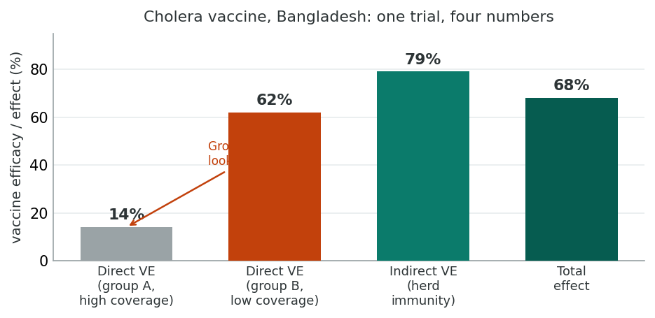
Example 12.7: Cholera Vaccine Effects in Bangladesh
Ali and colleagues (2005) and Hudgens and Halloran (2008) analysed an individually randomised, placebo-controlled trial of killed oral cholera vaccines in residential areas (baris) in Bangladesh. Two groups were compared: Group A (more than 50% coverage) and Group B (less than 28% coverage). The first-year risks per 1,000 were: RnvB = 7.01, RvB = 2.66, RnvA = 1.47, RvA = 1.27, RB = 4.13, RA = 1.34. Here each first-year risk R plays the role of the incidence I in the equations above, so the two symbols refer to the same quantity.
Direct effect in the high-coverage group A: VEd = (1.47 − 1.27) / 1.47 = 0.14. Looking at A alone you might conclude the vaccine has little effect.
Direct effect in the low-coverage group B: VEd = (7.01 − 2.66) / 7.01 = 0.62, so the vaccine reduces risk by 62% in the unprotected population.
Indirect effect (in the unvaccinated): (7.01 − 1.47) / 7.01 = 0.79, so herd immunity reduced the unvaccinated risk by 79%.
Total relative effect: (7.01 − 1.27) / 7.01 = 0.82. Overall effect: (4.13 − 1.34) / 4.13 = 0.68.
The lesson is striking: limiting analysis to the high-coverage population alone (Group A) would have suggested the vaccine barely worked. Looking across populations with different coverage reveals the dominant role of indirect effects.
Designing Vaccine Trials to Estimate All Three Measures
To estimate VEd, VEind, and VEtot, the design must include at least two comparable populations with different vaccination coverage. The recommended approach: in population A, randomise individuals to vaccine or placebo. In population B, leave everyone unvaccinated (or assign a lower coverage). The two populations must be (a) comparable in characteristics that affect the outcome, especially baseline transmission level, and (b) physically separated so subjects do not intermix.
An alternative when finding two similar populations is impractical is to exploit natural clustering, for example randomly assigning vaccination to half the children in a geographic area, then study spread within schools, recording the proportion of children at each school who were vaccinated. Riggs and Koopman (2005) and Longini and colleagues (1998, 2002) describe how to design and analyse such trials.
Reporting: The CONSORT 2010 Checklist
The CONSORT 2010 statement is the dominant reporting guideline for parallel-group randomised trials. Its 25 items align with the design and conduct topics covered throughout this lesson. The table below highlights items most relevant to the topics we have studied.
| Section / Item | What to Report |
|---|---|
| 1a Title | Identify the study as a randomised trial in the title (improves “searchability”). |
| 2a–b Background & objectives | Scientific rationale and explicit hypotheses or objectives. |
| 3a Trial design | Type of design (parallel, factorial, cross-over, cluster, split-plot) and allocation ratio. |
| 4a–b Participants | Eligibility criteria; settings and locations of data collection. |
| 5 Interventions | Sufficient detail for replication, including how and when administered. |
| 6a–b Outcomes | Pre-specified primary and secondary outcomes and how they were assessed. |
| 7a–b Sample size | How sample size was determined; explanation of any interim analyses or stopping guidelines. |
| 8–10 Randomisation | How the allocation sequence was generated, what type of restriction (blocking) was used, the mechanism for implementing allocation, and who did what at enrolment. |
| 11a–b Blinding | Who was blinded after assignment (participants, providers, outcome assessors); description of intervention similarity if relevant. |
| 12a–b Statistical methods | Methods for primary and secondary outcomes; methods for subgroup and adjusted analyses. |
| 13a–b Participant flow | For each group, numbers randomly assigned, receiving intended treatment, and analysed; losses and exclusions with reasons. A flow diagram is strongly recommended. |
| 14a–b Recruitment | Dates of recruitment and follow-up; reasons the trial ended or was stopped. |
| 15 Baseline data | Table of baseline demographic and clinical characteristics for each group. |
| 16 Numbers analysed | For each group, denominators in each analysis and whether by originally assigned groups. |
| 17a–b Outcomes & estimation | Effect size and precision (e.g., 95% CI); for binary outcomes, both absolute and relative effect sizes. |
| 18 Ancillary analyses | Other analyses (subgroup, adjusted), distinguishing pre-specified from exploratory. |
| 19 Harms | All important harms or unintended effects in each group. |
| 20–22 Discussion | Limitations (bias, imprecision, multiplicity); generalisability; interpretation balanced against benefits and harms. |
| 23–25 Other | Trial registration number; where the full protocol can be accessed; sources of funding and role of funders. |
CONSORT extensions exist for cluster randomised trials, non-inferiority and equivalence trials, non-pharmacological treatments, herbal interventions, and pragmatic trials. Up-to-date references are available at www.consort-statement.org.
Why Reporting Quality Matters
Poor reporting prevents readers from judging the reliability and validity of trial findings, prevents extraction for systematic reviews, and is associated with biased estimates of treatment effects. Inadequate reporting is therefore a methodological problem, with consequences beyond style. Following CONSORT during planning, and through to write-up, helps ensure that the methodological choices required for transparent reporting are actually made.
Reflection: Designing Your Own RCT
Imagine you have been funded to design a randomised controlled trial of a new mobile-app-based behavioural intervention to reduce daily smoking among young adults aged 18–25 living in rural communities. Briefly outline how you would address: (1) target population vs. source population vs. study group; (2) choice of allocation strategy (individual? cluster? factorial?); (3) choice of comparator (no app? sham app? existing standard care?); (4) how you would handle the analysis if compliance with the app turned out to be poor. Identify at least one trade-off you would face and explain how you would resolve it.
Minimum 20 characters required.
Key Takeaways
- Rigorous and equal follow-up of all groups is essential. Document compliance and reasons for withdrawal; a CONSORT flow diagram is strongly recommended.
- Intent-to-treat analysis preserves randomisation and gives a conservative, real-world estimate; per-protocol analysis estimates the effect under ideal compliance and should be reported alongside ITT, not in place of it.
- Multiple comparisons inflate the experiment-wise error rate. The Bonferroni adjustment (α / k) is the simplest correction. Subgroup analyses should be pre-specified and tested via interaction terms; data-driven subgroup analyses generate spurious findings.
- For prophylactic vaccines, three measures matter: direct (VEd), indirect or herd-immunity (VEind), and total (VEtot) efficacy. Estimating all three requires data from at least two populations with different coverage.
- The CONSORT 2010 checklist of 25 items structures both the planning and the reporting of randomised trials. Following CONSORT from the design stage through to write-up is what makes transparent reporting achievable.
1. The major reason that intent-to-treat analysis is preferred as the primary analysis is that:
2. In a vaccine trial, the indirect vaccine efficacy (VEind) is estimated by:
3. With four pre-specified primary outcome comparisons and a desired family-wise error rate of 0.05, the Bonferroni-adjusted significance threshold for each comparison is:
✦ Complete the reflection and pass the knowledge check with 100% to continue
Knowledge Check & Final Assessment
⏱ Estimated time: 15 minutes
Bringing It All Together
This lesson moved from observational into experimental epidemiology. You worked through the rationale for randomised controlled trials, the five phases of clinical research, the practical mechanics of allocation and masking, and the analytic and reporting standards (intent-to-treat, CONSORT 2010) that govern modern trial conduct. The shift from observational to experimental is conceptually small, since the investigator now assigns the exposure, but methodologically transformative, because randomisation is what gives RCTs their causal authority.
Together with the observational designs covered in earlier lessons and the hybrid designs covered in an earlier lesson, the controlled trial completes your toolkit of analytic study designs in epidemiology. The takeaways below summarise the design and reporting decisions that distinguish a credible trial from one that merely uses the word "randomised."
Key Takeaways from this lesson
- Randomisation is what makes the RCT the gold standard for causal inference: it balances measured and unmeasured confounders in expectation.
- Trial design begins with explicit target, source, and study populations, eligibility criteria, and a precisely specified intervention; vague specifications produce unreplicable results.
- Sample-size calculations must inflate for clustering by 1 + ρ(m − 1); sequential and adaptive designs change the inferential rules and require pre-specification.
- Allocation strategies (simple, stratified, cross-over, factorial, cluster, split-plot, multicentre) and masking (single, double, triple) each prevent specific biases.
- Intent-to-treat is the primary analysis because it preserves randomisation; per-protocol analyses are secondary and informative about efficacy under perfect compliance.
- Vaccine trials distinguish direct (VEd), indirect (VEind), and total (VEtot) efficacy; the CONSORT 2010 25-item checklist structures both planning and reporting of trials.
Reflection
Imagine you are leading a multidisciplinary team designing a randomised controlled trial of a community-level intervention to reduce opioid overdose deaths in a rural region. Drawing on what you have learned across this lesson, identify three design decisions you would face that involve trade-offs (for example: individual vs. cluster randomisation; placebo vs. active control; broad vs. narrow eligibility criteria). For each decision, briefly describe the trade-off, your recommended choice, and one specific limitation of that choice that you would acknowledge in your discussion of the trial.
Minimum 20 characters required.
Final Knowledge Assessment
Complete the following 12-question assessment. A score of 100% is required to complete the lesson. You may retake the assessment as many times as needed.
1. The defining feature that distinguishes a randomised controlled trial from an observational analytic study is that:
2. Phase III clinical trials are typically:
3. A trial's eligibility criteria that are very narrow will most likely:
4. In a cluster randomised trial of a school-based health programme with intra-cluster correlation ρ = 0.02 and an average cluster size of 51 students per school, the sample-size inflation factor is:
5. A factorial design is most appropriate when:
6. Triple-blinding adds which additional layer of masking compared with double-blinding?
7. The recommended primary analysis for a randomised controlled trial is:
8. With seven pre-specified primary outcome tests and a desired family-wise error rate of 0.05, the Bonferroni-adjusted alpha for each test is approximately:
9. Examining a wide range of post-hoc subgroups for differential treatment effects is risky because:
10. In a vaccine trial of two populations (Group A with high coverage, Group B with low coverage), which of the following is the formula for the indirect vaccine efficacy?
11. The Bangladesh cholera vaccine example (Example 12.7) illustrated that:
12. The CONSORT 2010 statement is:
✦ Complete the final reflection above before submitting