True OR
–
Evaluating Epidemiological Research
This course was developed by Dr. Kiffer G. Card, Faculty of Health Sciences, Simon Fraser University.
📚 Reference page, available throughout the lesson
This glossary collects the key concepts, people, and ideas you will meet in this lesson. Use it as a reference while you work through the material, or as a review before assessments. Type in the search box to filter entries.
An earlier lesson covered measurement validity and causal-specification mistakes; an earlier lesson covered selection biases that arise from who is in the study. This lesson takes the third leg of the standard bias triad: information bias, the systematic errors that arise from how exposure, outcome, and covariate data are recorded once participants are in the study (Sackett, 1979). The three content sections work through it from broad to specific. This section covers the misclassification framework that organizes all of information bias, distinguishes nondifferential from differential errors, and addresses the equity question of whose data are systematically wrong; a later section looks at observer and detection biases, errors that emerge from the data collector or the surveillance system rather than from the participant; a later section takes on regression dilution and digit preference, the more technical measurement artifacts that show up even when nobody is misclassifying anything. By the end of the lesson, you will have the third bias category in place; a later lesson then turns to design-specific and temporal biases that combine the three categories in characteristic ways.
Information bias (also called measurement bias or misclassification bias) occurs when exposure, outcome, or covariate data are systematically inaccurate. Unlike selection bias, which distorts who is in the study, information bias distorts what we know about the people in the study. It is one of the most pervasive threats to validity in epidemiological research because some degree of measurement error is present in virtually every study (Sackett, 1979; Hutcheon, Chiolero, & Hanley, 2010).
Information bias arises when the information collected about study participants is systematically inaccurate, leading to misclassification of exposure status, disease status, or both. The direction and magnitude of the resulting bias depend on whether the errors are the same across comparison groups (nondifferential) or differ between groups (differential).
Nondifferential misclassification occurs when the probability of being misclassified is the same for all study groups. This means that errors in measuring exposure are equally likely among cases and controls (or diseased and non-diseased), and errors in measuring outcome are equally likely among exposed and unexposed individuals.
Blair et al. (1996) compared two methods of assessing pesticide exposure in agricultural workers: self-reported exposure questionnaires and biological monitoring (urinary metabolite levels). Among workers reporting no pesticide exposure, approximately 30% had detectable urinary metabolites. Conversely, some workers reporting heavy exposure showed no biological evidence. When self-reported exposure was used to estimate associations with health outcomes, odds ratios were substantially attenuated compared to estimates using biomarker-based classifications.
When exposure is misclassified equally in both disease groups (for a binary exposure), the mixing of truly exposed and unexposed individuals in each category dilutes the true difference between groups. This generally attenuates (weakens) the observed association, biasing the odds ratio or relative risk toward 1.0. Because an odds ratio or relative risk of 1.0 means no association at all, biasing toward the null makes a real effect look weaker than it truly is, not stronger. However, for exposures with more than two categories, nondifferential misclassification can bias in either direction, and even for binary exposures the “always toward the null” rule can fail under correlated errors or extreme cell counts (Wacholder, 1995; Jurek, Greenland, Maldonado, & Church, 2005).
Nondifferential errors are the easier case: they typically pull effect estimates toward the null and do not flip the direction of an association. The harder case is when measurement quality itself depends on what we are trying to study.
Differential misclassification occurs when the accuracy of measurement differs between comparison groups. Unlike nondifferential misclassification, which typically biases toward the null, differential misclassification can bias results in either direction, toward or away from the null.
Two mothers, identical questions, different memories: watch differential recall create a fake association. Next ▶ advances scenes.
A 6-scene side-by-side of mothers in a birth-defect case-control study: the case mother who searches her memory for an explanation, the control mother who shrugs, and the resulting differential recall that inflates the odds ratio.
The INTERPHONE study (2010), a large multinational case-control study, investigated the association between mobile phone use and brain tumors. Cases (glioma and meningioma patients) reported their historical mobile phone use after diagnosis. A key finding was that cases with tumors on the same side of the head as their reported phone use showed a significantly elevated risk (OR = 1.8 for glioma), while cases with tumors on the opposite side showed a protective association (OR = 0.7). This implausible laterality pattern strongly suggests that cases differentially recalled or reported phone use on the side of their tumor, inflating the apparent association.
Recall Bias in Studies of Congenital Anomalies: Werler et al. (1989) demonstrated that mothers of children with birth defects recalled and reported medication use, dietary exposures, and environmental contacts more completely than mothers of healthy children. Mothers of affected infants were more likely to recall minor illnesses, prescription drug use, and chemical exposures during pregnancy. This differential recall inflates associations between reported exposures and congenital anomalies in case-control studies.
Swan et al. (1992) found that mothers of malformed infants reported 40% more occupational chemical exposures compared to what was documented in employment records, while mothers of healthy infants showed no such reporting excess.
Why does recall differ between cases and controls?
Strategies to reduce recall bias:
Recall bias (Coughlin, 1990) is one of two major mechanisms by which differential misclassification gets into a case-control study. The second is more general: participants distorting their answers in either direction depending on whether the answer is socially acceptable.
Midanik (1982) demonstrated that self-reported alcohol consumption in population surveys systematically accounts for only 40–60% of known alcohol sales in the same population. More recent studies using biomarkers such as phosphatidylethanol (PEth) confirm substantial underreporting: Kilian et al. (2020) found that biomarker-based estimates of heavy drinking prevalence were approximately twice as high as self-reported estimates. This underreporting is not random; it is most pronounced among heavy drinkers and in populations where drinking carries greater social stigma.
What you'll do: the simulator below holds a true population fixed and lets you set the sensitivity and specificity for measuring exposure and outcome separately, then toggle between non-differential and differential errors. Here sensitivity is the chance that someone who truly has the trait (exposed, or diseased) is recorded as having it, and specificity is the chance that someone who truly lacks it is recorded as lacking it; the same pair you met for screening tests, now describing how faithfully a study records its own variables. What to take away: the “always toward the null” rule for non-differential misclassification is approximate; it usually holds but can break in extreme cell counts; differential errors can move the OR in either direction by sizeable amounts. After working through the presets (especially Recall bias and Diagnostic suspicion), the equity discussion that follows asks who is most often subject to which kind of error.
A study of 1,000 people with a true exposure–outcome relationship. Now imperfect measurement shifts some people across cells. Drag sensitivity and specificity for exposure and outcome measurement, toggle whether errors are differential (depending on the other variable) or non-differential, and watch the observed effect drift.
Top: true counts. Bottom: what the study records.
| TRUE | ||
|---|---|---|
| Y+ | Y− | |
| E+ | – | – |
| E− | – | – |
| OBSERVED (with errors) | ||
|---|---|---|
| Y+* | Y−* | |
| E+* | – | – |
| E−* | – | – |
The misclassification framework above treats measurement error as a technical problem to be quantified and corrected. That framing is necessary but incomplete. Errors are not distributed at random across the population; they cluster along the same lines that structure inequality, and the way we choose to measure (or not measure) particular groups encodes a theory about whose health matters and whose suffering counts.
What gets measured shapes what knowledge is produced and how it is understood. Conversely, what is not measured, or measured badly, or with categories that erase relevant differences, becomes invisible to policy and intervention. The question “is this measurement biased?” is therefore inseparable from the question “biased relative to what underlying theory of disease, of population, and of justice?” (Krieger, 2011; Bauer, 2014).
Several of the biases discussed earlier in this section have a structural pattern that is easy to miss when they are presented as generic methodological problems:
Death certificates are the bedrock of mortality surveillance, but their accuracy is patterned. Studies comparing certificates with autopsy or chart review consistently find that “garbage codes” (ill-defined causes such as “cardiac arrest, unspecified”) are more common for decedents who are older, lower-income, racialised, or rural (Naghavi et al., 2010). Because cause-specific mortality drives both research priorities and resource allocation, differential misclassification at the certificate stage propagates inequities through every downstream analysis.
Race/ethnicity is recorded inconsistently across health systems: by self-report on some forms, by clinician observation on others, by next-of-kin on death certificates, and frequently as a single “Other” bucket that collapses dozens of communities. Indigenous identity in particular is systematically under-recorded. In Canada, Smylie and Firestone (2015) document substantial mismatches between First Nations, Métis, and Inuit self-identification and the way these populations appear (or fail to appear) in administrative health data.
The methodological consequence is differential misclassification of group membership, which can either deflate or inflate observed disparities depending on direction. The political consequence is that populations rendered statistically invisible struggle to make claims on a public health system that does not see them.
Most large health surveys until very recently collected only binary sex and no measure of gender identity or sexual orientation. Trans, non-binary, and Two-Spirit individuals have therefore been either invisible or actively miscoded, assigned to a category that does not match their lived identity, sometimes against their will (Bauer et al., 2009). When researchers later study, say, mental health by gender, the resulting estimates are imprecise, and worse, they are produced by an instrument that never asked the question.
Even when measurement instruments work well, populations who are systematically under-sampled cannot benefit from the resulting evidence. Clinical trials have historically over-represented White men of working age (Geller et al., 2018), genome-wide association studies have over-represented people of European ancestry (Sirugo, Williams, & Tishkoff, 2019), and pulse oximeters were calibrated on majority-White cohorts and over-estimate oxygen saturation in patients with darker skin (Sjoding et al., 2020). Each of these is a data-quality problem with equity stakes: the “noise” in the system is not symmetrically distributed.
Sjoding et al. (2020) compared paired pulse oximetry and arterial blood gas measurements in over 10,000 patients. Among Black patients, the pulse oximeter reported a saturation of 92–96% in 11.7% of cases when the true arterial saturation was below 88%, nearly three times the rate of occult hypoxemia observed in White patients (3.6%). During the COVID-19 pandemic, this calibration error meant that Black patients were systematically less likely to be flagged for supplemental oxygen, hospital admission, or therapy thresholds keyed to oximetry readings.
This is not a problem of human reporting bias or missing data. It is a problem of an instrument whose training conditions encoded a theory about the relevant patient population, and whose deployment in a more diverse population produced systematic, racially patterned misclassification.
Information bias is usually presented as something to be quantified and corrected: validation substudies, sensitivity analyses, regression calibration, multiple imputation. These tools are valuable, but they cannot fix a problem that lives in the categories themselves. If a survey collapses fifteen Indigenous nations into a single checkbox, no amount of post-hoc adjustment will recover the differences that were never captured. Fundamental causes of disease, social conditions that shape exposure to multiple risk factors and access to multiple resources, cannot be measured by instruments that were not designed to see them (Phelan, Link, & Tehranifar, 2010).
When you read a study and ask “is this measurement valid?”, also ask: Which populations were the instruments developed and validated in? Which categories are present and which are missing? Which differences are the analyses able, or unable, to detect? A null finding produced by a blunt instrument is not the same as evidence of no effect; it is evidence that this particular measurement system could not see one.
What you'll do: simulate a 10,000-person cohort with a true risk ratio of 2.0 (exposed risk = 0.20, unexposed risk = 0.10). Then apply (1) symmetric non-differential misclassification of exposure (20% flip rate in both groups) and (2) differential misclassification, where the recording error depends on disease status so that diseased people over-report exposure (a recall-bias analogue), and recompute the RR.
What to take away: non-differential misclassification pulls the RR toward the null (1.0); differential misclassification can move it in either direction. The simulation shows both.
set.seed(230)
n <- 10000
exposed <- rbinom(n, 1, 0.5)
# True risks: 0.20 in exposed, 0.10 in unexposed -> true RR = 2.0
disease <- rbinom(n, 1, prob = ifelse(exposed == 1, 0.20, 0.10))

# Truth from clean data
risk_t <- tapply(disease, exposed, mean)
risk_t["1"] / risk_t["0"]                  # ~ 2.0

# Non-differential misclassification of EXPOSURE (20% flipped each way)
flip <- rbinom(n, 1, 0.20)
exposed_obs <- ifelse(flip == 1, 1 - exposed, exposed)

risk_o <- tapply(disease, exposed_obs, mean)
risk_o["1"] / risk_o["0"]                  # attenuated < 2.0

# Stretch: DIFFERENTIAL misclassification (a recall-bias analogue).
# Now the error depends on DISEASE status, not exposure: diseased
# people over-report exposure, so truly-unexposed cases are recorded
# as exposed more often (25%) than truly-unexposed non-cases (5%).
fp_rate <- ifelse(disease == 1, 0.25, 0.05)
over_report <- rbinom(n, 1, fp_rate)
exposed_d <- ifelse(exposed == 1, 1, over_report)
risk_d <- tapply(disease, exposed_d, mean)
risk_d["1"] / risk_d["0"]Reading the three RRs. Clean RR ~ 2.0. Symmetric 20% misclassification of a binary exposure shrinks the RR toward 1.0 by mixing true exposed and unexposed people into each observed category. The differential run keys the error to disease status, so diseased people over-report exposure; that pushes the RR the other way, above the true value of 2.0 and away from the null. Non-differential error attenuates toward the null; differential error can move the estimate in either direction, depending on which outcome group is measured less accurately.
Use the questions below to interpret the output you produced. Look at your console before answering.
1. The clean-data RR was approximately 2.0 (the truth). After 20% non-differential misclassification, what RR did you get? In which direction did the bias move, toward 1.0 (the null) or away from it?
2. Why does symmetric misclassification of a binary exposure always pull the RR toward 1.0? Use the structure of the simulation (flipping 20% of true-exposed people into the "observed unexposed" group and vice versa) to explain.
3. The differential simulation (diseased people over-report exposure) pushed the RR away from the truth. This mirrors a case-control study where cases (sick people) recall exposures more thoroughly than controls. Name that classic bias and predict, with reference to your simulation, which direction the observed OR would move relative to the truth.
| Type | Error Pattern | Likely Bias Direction | Example |
|---|---|---|---|
| Nondifferential (binary) | Equal in both groups | Toward the null | Self-reported pesticide exposure |
| Nondifferential (polytomous) | Equal in both groups | Either direction | Dietary intake categories |
| Differential: recall bias | Cases recall more | Away from the null | Maternal exposure and birth defects |
| Differential: social desirability | Stigma-driven underreport | Depends on group | Alcohol and liver disease |
1. In the INTERPHONE study, the implausible laterality pattern (elevated risk on the same side as the tumor, protective effect on the opposite side) is best explained by:
2. A cohort study uses self-reported dietary questionnaires to assess red meat consumption and its association with colorectal cancer. Measurement error in the dietary questionnaire is equally likely among individuals who do and do not develop cancer. This will most likely:
3. Population surveys consistently find that self-reported alcohol consumption accounts for only 40–60% of known alcohol sales. If this underreporting is more pronounced among heavy drinkers than light drinkers, this represents:
An earlier section covered errors that originate with the participant: how they remember, how they report, how they answer sensitive questions. This section turns to errors that originate with the people and systems doing the measuring. The two halves of the section work through them in order: observer bias, where the data collector's knowledge of group assignment influences what gets recorded; and detection / surveillance bias, where one group is simply more likely to have its outcomes found because more eyes are looking. Both are rampant in screening studies and in observational comparisons of treated versus untreated patients.
Observer bias occurs when the person collecting or interpreting data is influenced by knowledge of participants’ exposure or disease status. When an observer knows which group a participant belongs to, their measurements, classifications, or interpretations may be unconsciously (or consciously) influenced, leading to systematic error.
Observer bias (also called ascertainment bias or interviewer bias) arises when an investigator’s awareness of a participant’s exposure or disease status systematically affects data collection (Sackett, 1979). The primary prevention strategy is blinding: ensuring that data collectors, outcome assessors, and analysts are unaware of group assignments.
Following widespread adoption of PSA (prostate-specific antigen) screening in the late 1980s, prostate cancer incidence in the United States increased dramatically, from approximately 100 per 100,000 men in 1986 to over 230 per 100,000 in 1992 (Etzioni et al., 2002). However, prostate cancer mortality changed very little during this period. The apparent “epidemic” was largely a detection artifact: intensive screening identified a reservoir of slow-growing, clinically insignificant cancers that would never have caused symptoms or death. This overdiagnosis created the illusion of both increased incidence and improved survival (lead-time bias).
Detection bias occurs when the probability of detecting a condition differs between comparison groups or changes over time due to differences in diagnostic intensity rather than true disease frequency. Key mechanisms include:
Together, these biases can make a screening program appear highly effective even when it provides minimal mortality benefit.
Two major randomized trials have produced conflicting results on PSA screening:
The discrepancy illustrates how detection bias complicates interpretation: the true effect of screening is difficult to isolate from the artifacts created by differential detection intensity.
Detection bias dominates discussions of screening. The same logic appears in every observational comparison of treated and untreated patients, where the treated group inevitably sees clinicians more often.
Surveillance bias is a form of detection bias that occurs when one exposure group receives more frequent medical monitoring than another, leading to differential detection of outcomes.
Women taking hormone replacement therapy (HRT) in observational studies typically had more frequent physician visits and mammographic screening than non-users. Haut et al. (2012) demonstrated that this differential surveillance explained a substantial portion of the observed association between HRT and breast cancer in early observational studies: HRT users were more likely to have breast cancer detected at earlier stages, not necessarily more likely to develop it. When analyses accounted for screening frequency, the apparent increased risk was substantially attenuated.
When you observe an association between an exposure and a disease outcome, ask: “Could this association be explained by differential detection rather than a true biological effect?” Key indicators of detection bias include:
Consider a cohort study examining whether people with diabetes have a higher incidence of depression compared to people without diabetes. People with diabetes visit their physicians more frequently and are routinely screened for depression as part of diabetes management. How might surveillance bias affect the observed association? What study design features could help disentangle true incidence from detection artifacts?
1. Following widespread PSA screening adoption, prostate cancer incidence doubled while mortality barely changed. The most accurate interpretation is:
2. In observational studies of HRT and breast cancer, the finding that HRT users had more frequent mammographic screening compared to non-users suggests that the observed association may be partly attributable to:
3. Which of the following is the most effective strategy for preventing observer bias in outcome assessment?
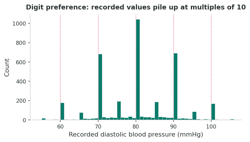
Recorded values cluster at numbers ending in 0 or 5 because of human rounding habits.
Myers (1940), Whipple (1919): age pyramids show saw-tooth patterns with excess counts at ages 30, 35, 40, 45, and 50.
Mant et al. (2006): 40 to 60% of clinical readings ended in zero. Expected rate: about 10%. Automated devices reduce this substantially.
Earlier sections worked on misclassification and detection, errors of which category a person ends up in. This final section addresses errors that arise even when nobody is misclassified. They come from the way values get recorded: a single noisy reading standing in for a true average, or numbers rounded toward preferred digits. These look small but their cumulative effect on the published literature has been documented to be large.
Regression dilution bias (also called regression attenuation bias) occurs when a single measurement of an exposure is used to represent a participant’s long-term or “usual” level (Hutcheon, Chiolero, & Hanley, 2010). Because any single measurement contains random within-person variation, the observed exposure distribution is wider than the distribution of true long-term values. This inflated variance dilutes the apparent exposure-outcome association.
Regression dilution bias arises when random within-person variation in a single baseline measurement underestimates the true association between a person’s usual exposure level and their risk of disease. The bias always attenuates the slope of the exposure-outcome relationship, making true associations appear weaker than they actually are.
MacMahon et al. (1990) demonstrated that studies using a single baseline blood pressure measurement substantially underestimated the association between usual blood pressure and stroke risk. The Prospective Studies Collaboration later showed that correcting for regression dilution approximately doubled the estimated effect: a 10 mmHg lower usual systolic blood pressure was associated with a 40% lower stroke risk, compared to the 20% apparent reduction from uncorrected single-measurement analyses. This correction was achieved by using repeat measurements from a sub-sample to estimate the ratio of between-person to total variance (the regression dilution ratio).
The Regression Dilution Ratio:
If the true association (slope) between usual exposure and log-risk is β, then the observed association from a single measurement is:
βobserved = λ × βtrue
where λ (lambda) is the regression dilution ratio:
λ = σ2between / (σ2between + σ2within)
Since λ is always between 0 and 1, the observed slope is always smaller than the true slope. Exposures with high within-person variability (e.g., dietary intake, blood pressure) have low λ values and severe regression dilution.
Nutritional Epidemiology: Regression dilution is particularly severe in dietary studies because single dietary assessments (24-hour recalls, food frequency questionnaires) have high within-person variability. Day-to-day variation in food intake means a single assessment poorly represents “usual” diet.
Willett (2013) showed that regression dilution ratios for single 24-hour dietary recalls range from 0.1 to 0.3 for many nutrients, meaning that observed diet-disease associations may represent only 10–30% of the true effect. This partly explains why nutritional epidemiology often produces weaker and more inconsistent findings than expected from biological plausibility.
Correction Methods:
Regression dilution is a problem of variance: how scattered values represent a stable true level. The next problem is about where values cluster, and why human rounding habits matter for analysis.
Digit preference (or heaping) occurs when recorded values cluster at certain numbers, typically those ending in 0 or 5, due to rounding by observers or self-reporters. While this may seem trivial, it introduces systematic measurement artifacts that can bias regression estimates and distort distributions.
Myers (1940) and Whipple (1919) demonstrated that census age data in many populations show pronounced heaping at ages ending in 0 and 5. In developing countries, this can be extreme: age pyramids show visible “saw-tooth” patterns where reported ages of 30, 35, 40, 45, and 50 have excess counts, while adjacent ages (29, 31, 34, 36) are depleted. This is quantified by Whipple’s Index, where a value of 100 indicates no heaping and 500 indicates all reported ages end in 0 or 5.
Quantifying the accuracy and agreement of measurement instruments is a prerequisite to interpreting any of the effect estimates below. The standard graphical and statistical approach to method comparison, plotting differences against means, was introduced by Bland & Altman (1986) and remains the default tool for validation substudies.
| Measurement Issue | Mechanism | Impact on Effect Estimates | Correction Strategy |
|---|---|---|---|
| Regression dilution | Within-person variability in single measures | Attenuates associations (bias toward null) | Repeat measures, calibration sub-studies |
| Digit preference | Rounding to preferred digits (0, 5) | Non-classical error; biases threshold-based analyses | Automated devices, statistical correction |
| Instrument drift | Equipment calibration changes over time | Time-varying systematic error | Regular calibration, quality control samples |
| Observer fatigue | Measurement quality degrades during long sessions | Increases random error; may become differential | Session limits, rest breaks, automated tools |
A researcher reports that a single baseline cholesterol measurement shows only a weak association (relative risk = 1.15 per mmol/L increase) with coronary heart disease over 10 years of follow-up. However, when the analysis corrects for regression dilution using repeat measurements, the association increases to RR = 1.45. Explain in your own words why the single-measurement estimate is biased and what the corrected estimate tells us. How should policymakers interpret the difference between these two estimates?
1. The Prospective Studies Collaboration found that correcting for regression dilution approximately doubled the estimated association between usual blood pressure and stroke risk. This correction was necessary because:
2. A vital statistics office finds that 52% of recorded birth weights end in “00” (e.g., 2500g, 3000g, 3500g), while only 10% would be expected if there were no digit preference. This heaping at the 2500g low-birth-weight threshold is most likely to:
3. A regression dilution ratio (λ) of 0.25 for dietary sodium intake from a single 24-hour recall means:
4. Which of the following is NOT an appropriate strategy for addressing digit preference in blood pressure measurement?
This lesson completed the third leg of the bias triad. An earlier section organized misclassification by whether errors are differential, traced its two main case-control mechanisms (recall and social desirability), and asked the equity question of whose data are systematically wrong. An earlier section turned to errors that originate with the data collector or the surveillance system: observer bias, detection bias in screening studies, and surveillance bias in comparisons of treated and untreated patients. An earlier section covered the quieter measurement artifacts, regression dilution and digit preference, that survive even when classification is accurate.
Read across the three sections, the unifying lesson is that information bias is not a single failure mode but a family of them, each demanding a different fix. Differential errors call for blinding and prospective designs; nondifferential errors call for better instruments or correction with validation sub-studies; ascertainment artifacts call for symmetric case-finding; regression dilution calls for repeated measures. The final reflection asks you to apply this full inventory to a single hypothetical study; the assessment then tests the conceptual content directly before the lesson hands off to a later lesson, where these errors combine with study-design choices in characteristic ways.
The companion R script r-activities/HSCI_230_Lesson_9_Information_Bias_and_Data_Quality.R simulates 10,000 individuals with a true risk ratio of 2.0, then flips 20% of exposure labels symmetrically in both directions and recomputes the observed RR, letting you watch non-differential misclassification pull the estimate toward the null in a single run.
set.seed(230)
n <- 10000
exposed <- rbinom(n, 1, 0.5)
# True risks: 0.20 in exposed, 0.10 in unexposed -> true RR = 2.0
disease <- rbinom(n, 1, prob = ifelse(exposed == 1, 0.20, 0.10))

# Truth from clean data
risk_t <- tapply(disease, exposed, mean)
risk_t["1"] / risk_t["0"]                  # ~ 2.0

# Add nondifferential misclassification of EXPOSURE (20% flipped each way)
flip <- rbinom(n, 1, 0.20)
exposed_obs <- ifelse(flip == 1, 1 - exposed, exposed)

risk_o <- tapply(disease, exposed_obs, mean)
risk_o["1"] / risk_o["0"] # attenuated < 2.0You are reviewing a case-control study that finds a strong association (OR = 2.5) between self-reported pesticide exposure and non-Hodgkin lymphoma. Cases were interviewed after diagnosis and asked to recall occupational exposures over the past 20 years. Controls were frequency-matched community members interviewed by telephone. Identify at least three distinct information biases that could threaten this study’s validity, explain the direction each would bias the results, and propose a specific design modification to address each one.
1. A cohort study uses self-reported smoking status (ever/never) to estimate the association between smoking and bladder cancer. Misclassification of smoking status is equally likely among those who do and do not develop bladder cancer. This nondifferential misclassification will most likely:
2. In a case-control study of birth defects, mothers of affected children report 40% more chemical exposures than documented in employment records, while mothers of healthy children show no such excess. This pattern is best described as:
3. A population survey of illicit drug use finds much lower prevalence rates when conducted via face-to-face interviews compared to audio computer-assisted self-interview (ACASI). The difference is most likely due to:
4. Following widespread adoption of PSA screening, prostate cancer incidence doubled while mortality remained relatively stable. This pattern is most consistent with:
5. In observational studies of statin use and cancer risk, statin users have significantly more frequent physician visits and blood tests than non-users. An observed positive association between statin use and cancer diagnosis should be interpreted cautiously because:
6. A researcher finds that a single baseline cholesterol measurement yields a relative risk of 1.15 per mmol/L for coronary heart disease, while regression dilution correction using repeat measurements increases this to RR = 1.45. The uncorrected estimate was biased because:
7. In a clinical setting, 55% of recorded blood pressure readings end in zero. This digit preference is most effectively addressed by:
8. A case-control study finds that cases with lung cancer recall significantly more occupational asbestos exposure than controls. However, when exposure is assessed using employer records, the association weakens considerably. The most likely explanation is:
9. Cotinine testing reveals that 12% of adults who report being non-smokers actually have cotinine levels consistent with active smoking. If these misclassified smokers are equally distributed among cases and controls in a case-control study of smoking and heart disease, this represents:
10. The regression dilution ratio for sodium intake measured by a single 24-hour dietary recall is approximately 0.20. To obtain an unbiased estimate of the association between usual sodium intake and blood pressure, a researcher should:
11. A blinded outcome assessor reviews MRI scans for a clinical trial comparing a new drug to placebo for multiple sclerosis. The assessor does not know which treatment each patient received. This blinding primarily prevents:
12. A study reports that birth weight data show pronounced heaping at 2500 grams. The researcher uses 2500g as a cutoff to define low birth weight. This analysis is problematic because: