Conceptualization, Measurement &
Causal Specification
Evaluating Epidemiological Research
Learning objectives for this lesson:
- Explain construct validity and identify threats such as measurement non-invariance and construct-irrelevant variance
- Distinguish between reliability and validity and describe how measurement error attenuates epidemiological associations
- Recognize when ordinal variables are inappropriately treated as interval-level data and the consequences for study findings
- Use directed acyclic graphs (DAGs) to identify collider bias, overadjustment bias, and confounding
- Explain the obesity paradox and smoking-birth weight paradox as examples of causal specification errors
- Distinguish residual confounding, reverse causation, and simultaneity bias using empirical examples
- Critically evaluate whether epidemiological studies have adequately addressed measurement and causal specification issues
This course was developed by Dr. Kiffer G. Card, Faculty of Health Sciences, Simon Fraser University.
Glossary: Key Terms, People & Concepts
📚 Reference page, available throughout the lesson
This glossary collects the key concepts, people, and ideas you will meet in this lesson. Use it as a reference while you work through the material, or as a review before assessments. Type in the search box to filter entries.
Construct Validity & Measurement
Ordinal is not interval; noise attenuates
Ordinal ≠ interval
Treating Likert categories as equally spaced can bias estimates and even reverse effect directions (Liddell & Kruschke, 2018).
Attenuation bias
Random measurement error in the exposure pulls the estimated slope toward zero. Reliability coefficients as low as 0.4–0.6 on food-frequency questionnaires help explain decades of apparent null findings in nutritional epidemiology.
Introduction and Overview
Earlier lessons surveyed the four observational designs and showed that each one is built on the same kind of 2×2 table with the same kind of measure of association. The unstated assumption running through all of those lessons is that the variables in the table actually mean what we think they mean: that “exposure” really is exposure, “disease” really is disease, and the chosen confounders are the right ones in the right relationship to the exposure and outcome. This lesson stops to interrogate that assumption. The three content sections each pick at a different layer of it: this section asks whether our instruments measure the constructs we say they measure (and whose theory of disease determined what got measured at all); a later section uses directed acyclic graphs to expose the most common causal-specification mistakes, such as conditioning on colliders, adjusting for mediators, and the “paradoxes” both produce; a later section works through three biases that survive even careful measurement and adjustment: residual confounding, reverse causation, and simultaneity. By the time you reach the sampling and selection, the inventory of biases this lesson opens will be ready to be combined with the additional biases that arise from who ends up in the study at all.
Learning Objectives
- Define construct validity, reliability, measurement non-invariance, and construct-irrelevant variance, and explain how each can bias an epidemiological study.
- Explain why measurement is theory-laden, that is, how the choice of biomedical, social-determinants, fundamental-causes, or ecosocial frameworks shapes which variables are measured at all.
- Apply Krieger’s and Link & Phelan’s arguments to predict what a study’s evidence base will and will not be able to see.
- Treat the choice of which population subgroups to disaggregate as a substantive theoretical decision, not a reporting afterthought.
- Recognise classical (random) measurement error and its tendency to attenuate associations toward the null (regression dilution bias).
Why Measurement Matters in Epidemiology
Epidemiological research depends on our ability to accurately measure the constructs we study, namely exposures, outcomes, and confounders. When measurements fail to capture the underlying phenomenon of interest, even a perfectly designed study can yield misleading results. This section examines how measurement problems introduce systematic error into epidemiological research.
Key Concept: Construct Validity
Construct validity refers to the degree to which a measurement instrument actually captures the theoretical concept it is intended to measure. A scale designed to measure “depression” has strong construct validity only if it truly reflects the underlying depressive construct rather than anxiety, fatigue, cultural distress, or social desirability.
Click each card below to explore the core measurement concepts that underpin epidemiological research.
Theory Before Instruments: How Frameworks Shape What We Measure
Construct validity asks whether an instrument captures the construct it is supposed to measure. A prior question is rarely asked but more consequential: where does the construct come from? Every variable in an epidemiological study is the residue of a theoretical decision, a claim about what causes disease, what counts as a relevant exposure, and where the boundary of the “cause” should be drawn. That decision is upstream of any psychometric work, and it determines what the rest of the analysis can possibly see.
Why this matters: measurement is theory-laden
What gets measured shapes what knowledge is produced and, by extension, what interventions become thinkable. If a study of cardiovascular disease measures cholesterol, blood pressure, and smoking but not neighbourhood disinvestment, occupational exposures, or experiences of discrimination, the resulting evidence base will reliably point clinicians toward statins and behavioural counselling rather than toward housing, labour, or anti-racism policy. The instruments did not pick themselves; a theory of disease causation picked them (Krieger, 2011).
Public health has historically been dominated by the biomedical model, which locates disease in individual bodies and explains population patterns as the aggregation of individual risk factors. The biomedical model is powerful for some questions (it gave us germ theory, vaccines, antibiotics), but it systematically under-measures the conditions in which bodies live, work, and age. Several theoretical frameworks have emerged to push back against this narrowness.
The social determinants of health framework, popularised by the WHO Commission on Social Determinants of Health (Solar & Irwin, 2010) and earlier by Marmot’s Whitehall studies (Marmot et al., 1991), holds that the conditions in which people are born, grow, live, work, and age are the dominant drivers of population health. Income, education, housing, food security, working conditions, and social inclusion explain a substantially larger share of the variance in health outcomes than medical care does (McGinnis, Williams-Russo, & Knickman, 2002).
If you accept this framework, your measurement priorities shift: a study of asthma incidence should measure mould exposure, landlord responsiveness, and traffic proximity alongside inhaler adherence.
Link and Phelan (1995) proposed that socioeconomic status is a fundamental cause of disease because it (1) influences multiple disease outcomes, (2) operates through multiple risk-factor mechanisms, (3) involves access to resources that can be deployed to avoid risks or minimise consequences, and (4) reproduces health inequalities even as the specific intervening mechanisms change over time.
This is why educational gradients in mortality have persisted across centuries even as the leading causes of death have shifted from infectious to chronic disease. The mechanism changed; the gradient did not. Measurement implication: adjusting for downstream behavioural mediators (smoking, diet) does not “explain away” the SES–mortality association, because flexible resources will simply find a new pathway. Treating SES purely as a confounder to be statistically controlled is a theoretical commitment, and arguably a mistaken one (Phelan, Link, & Tehranifar, 2010).
Nancy Krieger’s ecosocial theory asks how we “literally embody, biologically, the societal and ecological context into which we are born, develop, interact, and endeavor to live meaningful lives” (Krieger, 2001, p. 672). The theory unifies social and biological levels of analysis using the concept of embodiment: chronic exposure to discrimination, poverty, environmental hazards, and labour stress is literally inscribed in cortisol patterns, telomere length, allostatic load, and epigenetic marks.
Ecosocial theory pushes researchers toward measuring exposures across the lifecourse, at multiple spatial scales (body, neighbourhood, region, nation), and with explicit attention to power, history, and accountability for population health (Krieger, 2011).
Braveman (2014) defines health equity as the absence of unfair and avoidable differences in health among population groups defined socially, economically, demographically, or geographically. Equity is not the same as equality of average health; it is a claim about which differences are unjust.
Operationalising equity requires measuring along the axes where injustice is suspected to operate: race and income, and also Indigeneity, immigration status, gender identity, disability, and their intersections. A study that reports only an overall mean has, by omission, taken a position on which differences are worth noticing. Choosing not to disaggregate is itself a theoretical choice.
Imagine two research teams each studying type 2 diabetes incidence in the same population.
Team A works from a biomedical frame. They measure BMI, fasting glucose, HbA1c, dietary intake (FFQ), self-reported physical activity, and family history. Their conclusion: incidence is driven by individual lifestyle and genetic risk; intervention should target diet and exercise counselling.
Team B works from an ecosocial frame. They measure the same biomarkers and also neighbourhood food environment, shift-work history, lifetime experiences of racial discrimination, household income trajectory since childhood, and exposure to a major recession. Their conclusion: behavioural risk factors mediate roughly half of the social gradient; the rest reflects chronic stress and structural disinvestment. Intervention should include income support, labour protections, and neighbourhood investment alongside clinical care.
Both teams are doing “valid” epidemiology in the construct-validity sense. They reach different conclusions because they measured different things, and they measured different things because they began from different theories about what causes disease.
A caution and a balance
None of this means biomedical measurement is wrong. Cholesterol, viral load, and tumour staging are real, important, and often actionable. The argument is that biomedical models are frequently insufficient: they capture proximal mechanisms but obscure the upstream conditions that produce the patterns we observe. A defensible epidemiological study makes its theoretical commitments explicit, justifies its choice of constructs, and acknowledges what its instruments cannot see.
The four frameworks above name competing theories of what causes disease. The next case studies move from theory to instrument, showing how widely-used measurement tools quietly inherit the assumptions of whatever theory built them.
Case Study: The CES-D Scale and Differential Item Functioning
The CES-D is one of the most widely used screening instruments for depressive symptoms in population-based research. However, studies have documented significant differential item functioning (DIF) across racial, ethnic, and cultural groups. For example, Iwata et al. (2002) found that Japanese respondents endorsed somatic items (e.g., “my sleep was restless”) at higher rates than American respondents with equivalent levels of underlying depression, while American respondents endorsed affective items (e.g., “I felt sad”) at higher rates.
Similarly, Kim et al. (2011) demonstrated that multiple CES-D items function differently across non-Hispanic White, African American, and Hispanic adults in the United States. Items related to interpersonal difficulties showed DIF by race/ethnicity, meaning that a CES-D score of 16 (the traditional clinical cutoff) does not carry the same meaning across these groups.
Why This Matters for Epidemiological Research
When researchers compare depression prevalence across racial/ethnic groups using the CES-D, they may be comparing “apples to oranges.” Observed disparities in depression could reflect true differences in depressive symptomatology, differences in how groups express and report distress, or some combination of both. Without establishing measurement invariance, we cannot distinguish these explanations.
The CES-D case showed how a multi-item instrument can mean different things in different groups. The next example takes the same lesson to its limit: a single-item measure that turns out to be one of the strongest predictors in epidemiology, while inheriting all the same problems.
Self-Rated Health: A Deceptively Simple Measure
Self-rated health (SRH), typically measured as a single item (“How would you rate your overall health?”), is one of the strongest predictors of mortality in epidemiological research. Yet SRH responses are shaped by comparison groups, expectations, and cultural frameworks.
| Finding | Study | Implication |
|---|---|---|
| Lower-SES individuals report better SRH relative to their objective health indicators than higher-SES individuals | Sen (2002), Health: Perception versus Observation | SRH may underestimate health inequalities across socioeconomic strata |
| The predictive validity of SRH for mortality varies across racial/ethnic groups | Franks et al. (2003), Social Science & Medicine | Using SRH as a uniform outcome measure may introduce differential misclassification |
| Cultural differences in response styles (e.g., modesty norms) affect SRH reporting | Jylhä et al. (1998), Social Science & Medicine | Cross-national comparisons using SRH require careful calibration |
Validity questions about what we are measuring naturally lead to a related question about the scale on which we record the answer. Most epidemiological surveys use ordinal Likert-type response options; almost every analysis treats them as if the gaps between categories were equal. They usually are not.
The Problem of Scale Level: Ordinal vs. Interval
Epidemiological and health behavior research frequently uses Likert-type scales, which are ordinal response options such as “Strongly Agree” to “Strongly Disagree.” Researchers routinely assign numeric values (1–5) and analyze these as if the intervals between categories are equal. But is the “distance” between “Strongly Agree” and “Agree” really the same as between “Neutral” and “Disagree”?
The intuition in miniature: think of the order in which runners finish a race. Knowing that someone came first, second, or third tells you the ranking but not the gaps. First and second might be a hundredth of a second apart while third trails by a minute. Likert responses behave the same way. The labels are ordered, but the codes 1, 2, 3, 4, 5 we attach to them do not promise that each step is the same size on the underlying thing we care about.
Simulation studies by Liddell and Kruschke (2018) demonstrated that treating ordinal Likert data as metric (interval) in linear regression models can produce inflated Type I error rates, biased parameter estimates, and even reversals of effect direction. The bias is most severe when:
- Response distributions are skewed (e.g., most respondents cluster at one end of the scale)
- The spacing between response categories is unequal in the latent construct
- Interactions between variables are being tested
Appropriate alternatives include ordinal logistic regression or Bayesian ordinal models that respect the rank-order nature of the data.
Many large surveys measure physical activity using ordinal categories (e.g., “inactive,” “somewhat active,” “active,” “very active”). When researchers code these as 1–4 and fit linear models, they assume that the difference in health impact between “inactive” and “somewhat active” equals that between “active” and “very active.” In reality, evidence suggests the health benefits of physical activity follow a curvilinear pattern, with the largest gains at the lower end of the activity spectrum (Arem et al., 2015).
Construct validity, response-scale form, and cultural invariance are all about whether the instrument is asking the right thing. The last measurement issue this section covers is about whether it is asking it consistently.
Reliability and Attenuation Bias
Even when a measure is conceptually valid, poor reliability introduces random measurement error that systematically weakens (attenuates) observed associations. This is one of the most pervasive yet underappreciated problems in nutritional epidemiology.
Food frequency questionnaires (FFQs) are the most common method for measuring dietary intake in large cohort studies. However, test-retest reliability studies reveal substantial within-person variability. Willett (2013) demonstrated that single FFQ assessments can have reliability coefficients as low as 0.4–0.6 for many nutrients, meaning that 40–60% of the observed variance reflects random error rather than true between-person differences.
This measurement error leads to attenuation of diet-disease associations. For example, the true relative risk for the association between dietary fat intake and breast cancer risk may be 1.5, but observed relative risks in studies using FFQs might be only 1.1–1.2 due to regression dilution bias. This has contributed to decades of “null findings” in nutritional epidemiology that may reflect measurement limitations rather than true absence of effect (Kipnis et al., 2003).
Correction Methods
Researchers can use regression calibration and measurement error models to adjust for known attenuation. These methods require validation substudies with more precise measurements (e.g., biomarkers, doubly labeled water) to estimate the degree of measurement error and correct the observed associations (Carroll et al., 2006).
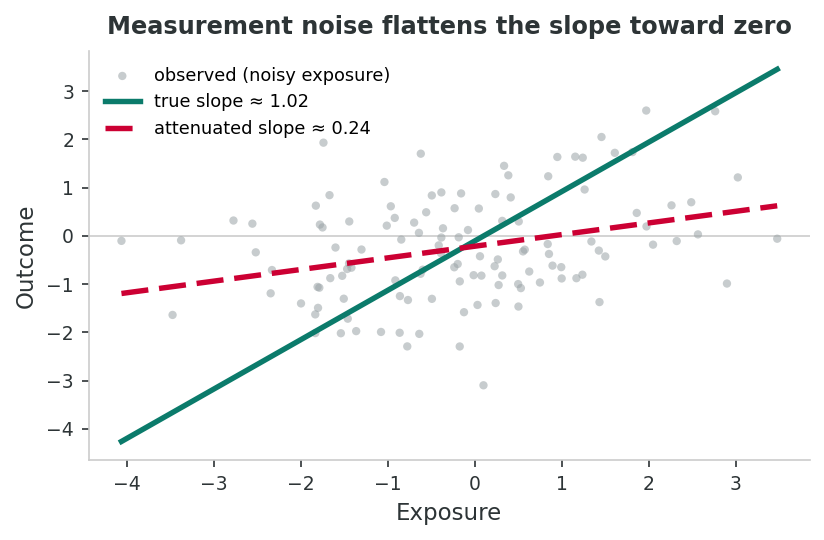
What you'll do: simulate 2,000 people with a true linear exposure-outcome slope of 1.0, then add measurement noise to the exposure and re-estimate the slope. Vary the noise size and watch the attenuation grow.
What to take away: random error in an exposure variable does more than add noise; it systematically pulls the estimated slope toward zero. The dirtier your instrument, the smaller your estimated effect.
set.seed(230)
n <- 2000

# True exposure X, outcome Y with true slope = 1
X <- rnorm(n, mean = 10, sd = 2)
Y <- 2 + 1*X + rnorm(n, sd = 1)

# Noisy version of X (e.g., FFQ-measured dietary intake)
X_noisy <- X + rnorm(n, sd = 2)

# Compare slopes from "perfect" vs "noisy" exposure
coef(lm(Y ~ X))["X"]               # expect ~1.00 (truth)
coef(lm(Y ~ X_noisy))["X_noisy"]   # expect < 1.00 (attenuated)

# Stretch: how does noise size change the attenuation?
sds <- c(0, 0.5, 1, 2, 4)
sapply(sds, function(s) {
  Xn <- X + rnorm(n, sd = s)
  unname(coef(lm(Y ~ Xn))[2])
})Reading the slopes. The clean regression recovers the true slope (~1.0). Adding noise with SD = 2 cuts the slope in half. Doubling noise SD to 4 shrinks it to ~0.2. This is exactly the mechanism that turns plausible diet-disease relationships into "null findings" when food-frequency questionnaires are the only exposure measure.
R Reflect on what you just ran
Use the questions below to interpret the output you produced. Look at your console before answering.
1. The true slope was 1.00. The clean lm(Y ~ X) recovered ~1.001 and the noisy lm(Y ~ X_noisy) recovered ~0.498. By what percentage was the noisy slope attenuated toward zero?
2. Read the stretch vector of slopes (sd = 0, 0.5, 1, 2, 4). Describe the pattern as measurement error SD grows. If a new biomarker cut measurement error SD from 2 down to 1, how close to the true slope of 1.0 would the new estimate get, based on your output?
3. Suppose X represents true dietary sodium and X_noisy represents self-reported FFQ-measured sodium. Connect your slope numbers to the Willett/Kipnis claim in this section: why might decades of "null findings" in nutritional epidemiology reflect measurement limitations rather than the absence of an effect?
Section Takeaways
- Every measured variable encodes a theoretical commitment about what causes disease; biomedical framings are powerful but often insufficient on their own.
- Frameworks such as the social determinants of health, fundamental causes, and ecosocial theory direct measurement toward upstream conditions that purely individual-level instruments cannot see.
- What gets measured shapes what becomes thinkable as an intervention, since omission is itself a theoretical choice, with implications for health equity.
- Construct validity determines whether we are measuring what we think we are measuring, a prerequisite for valid epidemiological inference.
- Measurement non-invariance means that identical scores may not be comparable across population subgroups.
- Treating ordinal data as interval can bias effect estimates and inflate false-positive rates.
- Poor reliability attenuates observed associations, potentially masking true causal effects.
1. A researcher finds that the CES-D depression scale yields different factor structures in African American versus non-Hispanic White adults. This is an example of:
2. A nutritional epidemiologist observes a relative risk of 1.15 for the association between dietary fiber and colorectal cancer, but the true relative risk is believed to be approximately 1.50. The most likely explanation for this discrepancy is:
3. A researcher assigns values of 1–5 to a Likert scale measuring perceived stress and fits a linear regression predicting blood pressure. Which assumption is most directly violated?
Causal Specification Errors
Introduction and Overview
An earlier section asked whether the variables in the table mean what we think they mean. This section asks whether we have put them in the right relationship to one another. The mistakes covered here, conditioning on colliders, adjusting for mediators, and mis-specifying the causal structure, do not show up in measurement error or sample size. They are mistakes about which variables to control for, and they can flip the sign of a true causal effect even when every measurement is perfect. The formal language for these decisions is the potential-outcomes framework (Rubin, 1974; Holland, 1986). The standard tool for thinking through these decisions is the directed acyclic graph (DAG); the standard takeaway is that more adjustment is not always better.
Learning Objectives
- Read and draw a directed acyclic graph (DAG) and identify confounders, mediators, and colliders within it.
- Explain why adjusting for a confounder removes bias, adjusting for a mediator removes part of the causal effect, and adjusting for a collider creates bias.
- Apply the back-door criterion to decide which variables to adjust for in a given DAG.
- Recognise the canonical “paradoxes” (e.g. obesity paradox, birthweight paradox) as collider-bias artefacts rather than real biological effects.
- Use a DAG to defend an analytic choice in plain language to a non-statistical collaborator.
Directed Acyclic Graphs (DAGs) for Causal Reasoning
A directed acyclic graph (DAG) (Pearl, 1995) is a visual tool that represents causal assumptions about the relationships among variables. Each arrow indicates a hypothesized direct causal effect. DAGs help researchers identify which variables to adjust for and, critically, which variables should not be adjusted for, to obtain unbiased causal estimates. The accordion below works through three canonical cases: confounding (where adjustment removes bias), collider bias (where adjustment creates it), and mediator adjustment (where adjustment removes part of the very effect you are trying to estimate). After the worked examples, the interactive playground that follows lets you build each pattern by clicking variables to adjust or not.
Three Key DAG Structures
Confounder: A variable that causes both the exposure and the outcome. Adjusting for a confounder removes bias. Example: Age → Physical Activity; Age → Heart Disease.
Mediator: A variable on the causal pathway between exposure and outcome. Adjusting for a mediator blocks part of the causal effect you are trying to estimate. Example: Smoking → Inflammation → Cancer.
Collider: A variable caused by both the exposure and the outcome (or by variables associated with each). Adjusting for a collider creates spurious associations where none existed. Example: Obesity → Hospitalization ← Cancer.
A note on vocabulary
Several phrases in this section describe the same underlying operation. Adjusting for a variable, controlling for it, conditioning on it, stratifying by it, and restricting the sample to one of its values all mean holding that variable fixed while you look at the exposure and the outcome. Whether doing so helps or hurts depends entirely on the variable's role in the diagram: it removes bias for a confounder, but it can create bias for a collider or a mediator.
Consider the association between coffee drinking and lung cancer. A naive analysis might suggest coffee increases cancer risk. However, a DAG reveals that smoking is a confounder:
Smoking → Coffee Drinking
Smoking → Lung Cancer
People who smoke are more likely to drink coffee. Failing to adjust for smoking creates a spurious association between coffee and cancer. Adjusting for smoking removes this confounding and the association typically disappears (Greenland et al., 1999).
Consider a study examining the relationship between talent and attractiveness among Hollywood actors. Both traits independently increase the chance of becoming famous:
Talent → Fame ← Attractiveness
Fame is a collider. If we restrict our analysis to famous people (i.e., condition on the collider), we create a spurious negative association: among famous people, those who are less attractive tend to be more talented, and vice versa. This is an artifact of the selection, not a real causal relationship (Elwert & Winship, 2014).
Suppose we want to estimate the total effect of education on mortality. Education may improve health through better employment and income:
Education → Income → Mortality
Education → Mortality (direct)
If we adjust for income (a mediator), we block the indirect pathway and estimate only the direct effect of education on mortality. If the research question asks about the total effect, adjusting for income leads to overadjustment bias, underestimating the true impact of education (Schisterman et al., 2009).
Hands-on: Causal DAG Playground
What you'll do: pick a scenario (confounding, collider, mediator, M-bias, instrumental variable, or the obesity-paradox case), then click each variable to toggle whether you would adjust for it. The simulator shows every backdoor path between exposure and outcome, marks each one as open or closed, and tells you whether the total causal effect is identifiable. What to take away: the canonical mistake in observational analysis is over-adjustment, that is, conditioning on variables that look like helpful controls but are actually colliders or mediators. After playing with each preset, the case studies that follow apply the same logic to two famous “paradoxes” in the published literature.
🔗 Interactive: Causal DAG Playground
Pick a scenario, then click each variable to adjust for it (or not). The tool shows every backdoor path between E and Y, whether your choice blocks or opens each path, and whether the total causal effect of E on Y is identifiable. The lesson: more adjustment is not always better, because conditioning on a collider opens a biasing path.
DAG
Paths from E to Y
The simulator builds the abstract patterns. The two case studies below show those patterns in action in the published literature: each “paradox” turns out to be the literature's name for what happens when investigators adjust for the wrong variable.
Case Study: The Obesity Paradox
Multiple observational studies have reported that among patients with chronic diseases such as heart failure, chronic kidney disease, and diabetes, overweight and obese patients appear to have better survival than normal-weight patients. This counterintuitive finding has been termed the “obesity paradox” and has generated considerable debate.
However, Banack and Kaufman (2014) demonstrated using DAGs and simulations that this paradox can be explained by collider stratification bias. When researchers restrict their analysis to patients already diagnosed with a chronic disease, they are conditioning on a collider:
Obesity → Chronic Disease ← Other Risk Factors (e.g., smoking, frailty)
Obesity → Mortality
Other Risk Factors → Mortality
Among the chronically ill, those who are normal weight are more likely to have the disease due to other severe risk factors (smoking, genetic susceptibility). Conditioning on chronic disease status induces a spurious protective association between obesity and mortality.
Critical Implication
The obesity paradox illustrates how inappropriate restriction or stratification can reverse the direction of a true causal effect. Studies that analyze only patients with a disease, without recognizing that the disease is a collider between the exposure and other causes of mortality, can produce deeply misleading conclusions with serious public health implications.
The obesity paradox is a collider problem. The next case is the closely related, and in some ways even more pernicious, mediator problem.
Case Study: Overadjustment Bias in Perinatal Epidemiology
Maternal smoking during pregnancy is a well-established cause of both low birth weight and infant mortality. However, several studies that adjusted for birth weight reported the puzzling finding that maternal smoking appeared to have a reduced or null association with infant mortality among low-birth-weight infants, the so-called “birth weight paradox.”
Hernandez-Diaz et al. (2006) used DAGs to show that this paradox arises from overadjustment. Birth weight is a mediator on the causal pathway from smoking to infant mortality:
Smoking → Low Birth Weight → Infant Mortality
Smoking → Infant Mortality (direct)
Birth Defects → Low Birth Weight → Infant Mortality
Adjusting for birth weight blocks the indirect causal path through which smoking increases mortality. Moreover, birth weight is also a collider between smoking and birth defects, so conditioning on it induces a spurious negative association between smoking and birth defects, making smoking appear protective among low-birth-weight infants.
Reflection
Think of a study you have encountered (in this course or elsewhere) that examined the association between an exposure and an outcome while adjusting for a variable on the causal pathway. Could this adjustment have introduced overadjustment bias or collider bias? Describe the variables and the potential DAG structure.
Section Takeaways
- DAGs are essential tools for identifying confounders, mediators, and colliders before analyzing data.
- Collider bias (conditioning on a common effect) can create spurious associations or reverse the direction of real effects.
- The obesity paradox is likely an artifact of collider stratification bias, not a true protective effect of obesity.
- Adjusting for mediators (e.g., birth weight when studying smoking and infant mortality) introduces overadjustment bias.
1. In a study of heart failure patients, researchers find that obese patients survive longer than normal-weight patients. According to the collider bias explanation, what variable is being inappropriately conditioned on?
2. In the birth weight paradox, adjusting for birth weight when estimating the effect of maternal smoking on infant mortality introduces bias because birth weight is a:
3. A researcher wants to estimate the total effect of education on cardiovascular mortality. Which of the following variables should NOT be adjusted for?
Residual Confounding, Reverse Causation & Simultaneity
Introduction and Overview
An earlier section covered measurement; an earlier section covered the structure of the causal model. This section addresses three biases that survive both. Residual confounding remains even after correct DAG specification, because we never measure confounders perfectly. Reverse causation arises when the apparent cause is actually downstream of the apparent effect. Simultaneity is the limit case where two variables cause each other and the very framing of the analysis is wrong. All three are common enough in the published literature that you will encounter examples within a few weeks of any reading list.
Learning Objectives
- Define residual confounding and explain why it persists even after “adjusting for” a confounder.
- Use the HRT–cardiovascular discordance to illustrate how imprecisely measured socioeconomic confounders can mimic large protective effects.
- Identify reverse causation in published associations and propose study designs (longitudinal data, instrumental variables, Mendelian randomisation) that can adjudicate it.
- Define simultaneity (mutual causation) and explain why standard regression adjustment cannot resolve it.
- Read an observational study with all three biases (residual confounding, reverse causation, simultaneity) on a checklist before believing its causal claim.
Residual Confounding
Residual confounding occurs when adjustment for a confounder is incomplete, either because the confounder is measured imprecisely, categorized too coarsely, or only partially captured by the available variables. Even when researchers “adjust for” a confounder, residual confounding can persist and bias effect estimates.
Definition: Residual Confounding
The bias that remains after adjustment for a confounder, due to imperfect measurement or incomplete capture of the confounding variable. It is a form of unmeasured confounding within measured variables.
Hormone Replacement Therapy and Cardiovascular Disease
For decades, observational studies consistently showed that postmenopausal women using hormone replacement therapy (HRT) had a 30–50% lower risk of cardiovascular disease (CVD) compared with nonusers. This finding influenced clinical guidelines worldwide.
However, the Women's Health Initiative (WHI) randomized trial found that HRT actually increased cardiovascular risk (Rossouw et al., 2002). What explained the discrepancy?
Subsequent analyses by Humphrey et al. (2002) and Hernan et al. (2008) showed that the observational studies suffered from residual confounding by socioeconomic status, healthy user bias, and smoking. Women who chose HRT were healthier, wealthier, and more health-conscious than those who did not, and even after adjusting for measured covariates, the adjustment was incomplete.
Why Adjustment Fails
Residual confounding arises through several mechanisms:
- Measurement error in the confounder: If smoking is measured as ever/never rather than pack-years, considerable confounding by smoking intensity remains unadjusted.
- Coarse categorization: Adjusting for income in broad categories ($0–$30K, $30K–$60K, $60K+) leaves within-category confounding by fine-grained socioeconomic differences.
- Omitted dimensions: “Socioeconomic status” encompasses education, income, wealth, occupational prestige, and neighborhood context. Adjusting for education alone leaves residual confounding by the other components.
Simulation studies by Fewell et al. (2007) demonstrated that even modest measurement error in a strong confounder can leave substantial residual confounding, sufficient to create or mask associations of the magnitude commonly reported in epidemiological research.
Addressing Residual Confounding
- Improve measurement: Use continuous rather than categorical measures of confounders when possible; use validated instruments with known measurement properties.
- Sensitivity analyses: Quantitative bias analysis (e.g., E-values) can estimate how strong unmeasured or residual confounding would need to be to explain away an observed association (VanderWeele & Ding, 2017).
- Negative control exposures/outcomes: Variables that should not be associated with the outcome (or exposure) can help detect residual confounding (Lipsitch et al., 2010).
- Triangulation: Compare results across study designs with different confounding structures (e.g., observational vs. Mendelian randomization).
Residual confounding is what is left over after we have tried to adjust for the variables we know about. The next bias is what happens when our entire ordering of cause and effect is wrong.
Reverse Causation
Reverse causation occurs when the presumed outcome actually causes (or influences) the presumed exposure, rather than the other way around. This is particularly problematic in cross-sectional and case-control studies where the temporal sequence of events is unclear.
Numerous observational studies report that physical inactivity is associated with increased risk of chronic diseases including cardiovascular disease, diabetes, and cancer. While this association is likely at least partly causal, reverse causation is a major concern: people who are developing chronic illness may reduce their physical activity because of early symptoms, fatigue, or functional limitations.
Ding et al. (2020) examined data from the UK Biobank and found that excluding the first several years of follow-up (to allow for a “lag period”) substantially attenuated the association between physical activity and mortality, consistent with reverse causation. Individuals who died early in follow-up were more likely to have been inactive at baseline because they were already sick.
Strategies to Address Reverse Causation
Lag analyses: Exclude events occurring in the first few years of follow-up to remove individuals whose exposure was influenced by pre-existing disease.
Prospective design with repeated measures: Track changes in exposure over time to determine temporal ordering.
Instrumental variable approaches: Use genetic variants (Mendelian randomization) that influence exposure but are not affected by disease status.
Reverse causation flips the direction of a single arrow. The third bias goes one step further: it allows arrows in both directions at once.
Simultaneity Bias
Simultaneity bias (also called bidirectional causation) arises when two variables mutually cause each other, making it impossible to identify the causal direction from observational data alone. Standard regression models assume that the predictor causes the outcome, not vice versa; when causation runs in both directions, ordinary regression estimates are biased.
The relationship between obesity and depression has been the subject of hundreds of studies. Meta-analyses by Luppino et al. (2010) found evidence for bidirectional causation:
- Obesity at baseline increased the risk of subsequent depression (OR = 1.55, 95% CI: 1.22–1.98)
- Depression at baseline increased the risk of subsequent obesity (OR = 1.58, 95% CI: 1.33–1.87)
This bidirectional relationship means that a cross-sectional study finding an association between obesity and depression cannot determine whether obesity causes depression, depression causes obesity, or both. Moreover, standard regression approaches that treat one variable as the “exposure” and the other as the “outcome” will produce biased estimates because each variable is both a cause and consequence of the other.
| Bias Type | Core Problem | Primary Study Design Vulnerability | Key Mitigation Strategy |
|---|---|---|---|
| Residual Confounding | Incomplete adjustment for measured confounders | All observational designs | Better measurement, sensitivity analysis, triangulation |
| Reverse Causation | Outcome influences exposure rather than vice versa | Cross-sectional, short-follow-up cohorts | Lag analyses, repeated measures, Mendelian randomization |
| Simultaneity | Two variables mutually cause each other | Cross-sectional, standard regression models | Longitudinal cross-lagged models, instrumental variables |
Reflection
Consider the finding that people who eat more fruits and vegetables tend to have lower rates of depression. Describe how residual confounding, reverse causation, and simultaneity could each offer alternative explanations for this association. Which do you think is most plausible, and why?
Section Takeaways
- Residual confounding persists even after statistical adjustment when confounders are measured imprecisely or categorized too coarsely.
- The HRT-CVD discrepancy between observational studies and the WHI trial is a landmark example of residual confounding by healthy user bias.
- Reverse causation is especially problematic in studies of physical activity and chronic disease, where declining health may reduce activity.
- Simultaneity bias arises when two variables are mutually causal (e.g., obesity and depression) and requires specialized analytical approaches.
1. Observational studies found that HRT reduced cardiovascular risk by 30–50%, but the WHI trial showed HRT increased risk. The most likely explanation for this discrepancy is:
2. A researcher observes that physically inactive individuals in a cohort study have higher mortality. To assess whether reverse causation might explain this finding, the most appropriate strategy would be:
3. The association between obesity and depression is bidirectional: obesity predicts future depression, and depression predicts future obesity. This is an example of:
4. A researcher adjusts for smoking using a binary variable (ever/never smoker) when studying the effect of air pollution on lung cancer. This adjustment is likely insufficient because:
Final Assessment
Bringing It All Together
This lesson took apart three of the deepest assumptions baked into every observational analysis: that the variables mean what we say they mean, that we have controlled for the right things in the right way (Hernán, 2004), and that the cause comes before the effect. Each section then built up the corresponding repertoire of biases: measurement (an earlier section), causal-specification (an earlier section), and the residual problems that survive both (an earlier section). Together they form a checklist you can apply to any study you read for the rest of this course and through later courses.
The deeper move was the one Krieger and Link & Phelan have been making for decades: instruments do not pick themselves. Whether a study can “see” structural racism, neighbourhood disinvestment, occupational exposure, or chronic discrimination depends entirely on which theoretical framework chose its variables in the first place. A perfectly executed analysis of variables drawn from the wrong framework will reliably produce evidence that points away from the actual drivers of population health. That is why the conceptualisation step matters before the measurement step, and the measurement step before the causal-specification step.
A later lesson takes the next layer: who ended up in the study at all. Sampling, selection, and external validity are the biases that arise from which subjects we get to observe, biases that combine with the measurement and causal-specification problems documented here to produce the final, integrated picture of why an observational study’s causal claim might be wrong.
Key Takeaways from this lesson
- Construct validity is theory-laden. The choice of which constructs to measure is a theoretical commitment that shapes which interventions ever become thinkable.
- Reliability and validity are not the same. A measure can be perfectly reliable and still capture the wrong construct; classical (random) error tends to attenuate associations toward the null.
- DAGs are the discipline of causal specification. Confounders should be adjusted for, mediators should not (if the total effect is the target), and colliders create bias when conditioned on.
- More adjustment is not always better. The “obesity paradox” and other apparent paradoxes are typically collider-bias artefacts produced by over-adjustment, not new biology.
- Residual confounding is the rule, not the exception. The HRT–cardiovascular discordance shows what happens when an imprecisely measured SES gradient is mistaken for a treatment effect.
- Reverse causation and simultaneity survive even careful measurement and DAG specification; resolving them requires longitudinal data, instrumental variables, or Mendelian randomisation, not more covariate adjustment.
This lesson took apart the assumptions baked into every observational analysis: that variables mean what we say they mean, that we have controlled for the right things in the right way, and that the cause comes before the effect. Each section then built up the corresponding repertoire of biases: measurement, causal-specification, and the residual problems that survive both. The reflection below asks you to put all three layers to work on a single hypothetical study; the comprehensive assessment that follows tests the conceptual material across the three sections.
The companion R script r-activities/HSCI_230_Lesson_7_Conceptualization_Measurement_and_Causal_Specification.R simulates a true linear association between an exposure and an outcome, then re-fits the model after adding classical measurement error to the exposure (e.g., a food-frequency questionnaire). You will see the regression slope shrink toward zero, the textbook signature of attenuation bias, and watch the shrinkage grow as the measurement-error SD increases.
set.seed(230)
n <- 2000

# True exposure X, outcome Y with true slope = 1
X <- rnorm(n, mean = 10, sd = 2)
Y <- 2 + 1*X + rnorm(n, sd = 1)

# Noisy version of X (e.g., FFQ-measured dietary intake)
X_noisy <- X + rnorm(n, sd = 2)

# Compare slopes from "perfect" vs "noisy" exposure
coef(lm(Y ~ X))["X"]             # expect ~1.00 (truth)
coef(lm(Y ~ X_noisy))["X_noisy"] # expect < 1.00 (attenuated)

## -----------------------------------------------------------------------------
## Stretch: how does noise size change the attenuation?
## -----------------------------------------------------------------------------
sds <- c(0, 0.5, 1, 2, 4)
sapply(sds, function(s) {
  Xn <- X + rnorm(n, sd = s)
  unname(coef(lm(Y ~ Xn))[2])
})
# Larger SD of measurement error -> larger attenuation toward zero.
Reflection
You are reviewing a study that reports a statistically significant association between a self-reported behavioral exposure (measured with a Likert scale) and a chronic disease outcome. Drawing on what you learned in this lesson, describe at least three distinct measurement or causal specification issues that could threaten the validity of this finding. For each, explain how the researchers might address it.
Final Knowledge Assessment
This 15-question assessment covers all topics from this lesson. You must score 100% to complete the lesson. Review the explanations for any incorrect answers and try again.
1. Construct validity refers to:
2. Differential item functioning on the CES-D across racial groups means:
3. Random measurement error in an exposure variable typically leads to:
4. A researcher fits a linear regression using a 5-point Likert scale as the predictor. The primary concern with this approach is:
5. In a DAG, a collider is a variable that:
6. The “obesity paradox” (apparent protective effect of obesity among chronically ill patients) is best explained by:
7. In the birth weight paradox, adjusting for birth weight when estimating the effect of smoking on infant mortality is problematic because:
8. Overadjustment bias occurs when a researcher adjusts for:
9. Residual confounding differs from unmeasured confounding in that:
10. The discrepancy between observational studies and the WHI trial regarding HRT and cardiovascular disease primarily illustrates:
11. In a cohort study, physically inactive people have higher mortality. Excluding deaths in the first 5 years of follow-up substantially attenuates this association. This suggests:
12. The finding that obesity predicts future depression AND depression predicts future obesity is an example of:
13. An E-value is used to:
14. Self-rated health (SRH) varies across socioeconomic groups even when objective health is similar. This is most directly a threat to:
15. A researcher studying diet and cancer adjusts for smoking using an ever/never variable instead of pack-years. The residual confounding from this approach will most likely: