RR within C+
–
Evaluating Epidemiological Research
This course was developed by Dr. Kiffer G. Card, Faculty of Health Sciences, Simon Fraser University.
📚 Reference page, available throughout the lesson
This glossary collects the key concepts, people, and ideas you will meet in this lesson. Use it as a reference while you work through the material, or as a review before assessments. Type in the search box to filter entries.
Earlier lessons worked through bias one category at a time. This lesson finishes the inventory by addressing the third leg of the canonical bias triad, confounding, and then steps back to the statistical-inference issues that turn even unbiased estimates into wrong conclusions. The two content sections divide the work cleanly. This section takes confounding from the textbook definition through pharmacoepidemiology's standard nightmare (confounding by indication), through the more advanced problem of time-varying confounding, into the harder theoretical question of whether constructs like race or income are confounders to be controlled or structural exposures to be measured. A later section turns to the analytic issues that haunt even well-adjusted models: model misspecification, multicollinearity, Type I/II errors, Simpson's paradox, the ecological fallacy, the modifiable areal unit problem, and missing data. By the end, the toolkit needed for a later lesson's integrated appraisal will be complete.
Confounding occurs when a third variable, the confounder, is associated with both the exposure and the outcome, distorting the observed relationship between them. Unlike mediators (which lie on the causal pathway), confounders represent alternative explanations for an association. If unaddressed, confounding can make a harmful exposure appear protective, a beneficial treatment appear harmful, or a null relationship appear significant.
A variable C is a confounder of the exposure–outcome relationship if it satisfies three conditions: (1) C is associated with the exposure, (2) C is an independent risk factor for the outcome (it raises or lowers outcome risk on its own, not only through the exposure), and (3) C is not on the causal pathway between the exposure and the outcome. If C is a mediator rather than a confounder, adjusting for it introduces bias rather than removing it. The modern formal definition is given by VanderWeele & Shpitser (2013), building on Greenland and Robins' (1986) foundational link between confounding, identifiability, and exchangeability; Hernán et al. (2002) further showed that confounder identification requires causal knowledge and not statistical association alone.
One of the most consequential examples of confounding in modern epidemiology involves hormone replacement therapy (HRT) and cardiovascular disease (CVD) risk in postmenopausal women. For decades, observational studies consistently suggested that HRT reduced CVD risk by 30–50%. These findings influenced clinical guidelines worldwide.
The WHI was a large randomized controlled trial launched in 1991. When results were published by the Writing Group for the WHI Investigators (2002), they revealed that combined estrogen–progestin therapy actually increased the risk of coronary heart disease (HR 1.29, 95% CI: 1.02–1.63), stroke, and pulmonary embolism. The discrepancy was explained by confounding by socioeconomic status and health behaviors: women who chose HRT in observational studies tended to be wealthier, better educated, leaner, more physically active, and more engaged with preventive healthcare, all factors independently associated with lower CVD risk. Reading the trial estimate: the 95% confidence interval (1.02 to 1.63) lies entirely above 1, the value that marks no effect, so the data are compatible only with increased risk, not with protection.
What you'll do: simulate a 5,000-person dataset in which HRT has zero effect on CVD, then watch how an SES confounder produces a misleading crude OR that disappears when you look within strata or adjust in regression. What to take away: stratification is the most direct demonstration of confounding: if the within-stratum estimates agree with each other but disagree with the crude estimate, you have confounding by the stratifying variable, and the within-stratum value is the unbiased one.
The classic remedy for confounding is to look within levels of the suspected confounder. The simulation below builds a true-null exposure-outcome relationship that's polluted by an SES confounder. The crude OR misleads; the stratum-specific ORs show the truth.
set.seed(230)
n <- 5000
ses <- rbinom(n, 1, 0.5)                                  # 1 = high SES
hrt <- rbinom(n, 1, prob = ifelse(ses == 1, 0.6, 0.2)) # high SES uses HRT more
# CVD risk: lower in high SES, NOT affected by HRT (true null)
cvd <- rbinom(n, 1, prob = ifelse(ses == 1, 0.05, 0.15))

# Crude (unadjusted) OR -- looks "protective"
exp(coef(glm(cvd ~ hrt, family = binomial))["hrt"])

# Within each SES stratum -- the true effect: ~1.0
tapply(seq_len(n), ses, function(i) {
  exp(coef(glm(cvd[i] ~ hrt[i], family = binomial))[2])
})

# Adjusted OR, controlling for SES
exp(coef(glm(cvd ~ hrt + ses, family = binomial))["hrt"])This is the WHI lesson in miniature. The crude estimate (about 0.61) sits well below 1; since an odds ratio below 1 means lower odds of disease, it reads as protection, exactly the kind of number that fed twenty years of observational HRT enthusiasm. Adjusting for SES recovers the true null, an odds ratio near 1. In a later course you will build this intuition with Mantel-Haenszel summaries; in a later course you will use multivariable regression.
Use the questions below to interpret the output you produced. Look at your console before answering.
1. The crude OR for HRT vs CVD was about 0.61 (well below 1), but the simulation built HRT with zero effect on CVD. Walk through the three conditions of confounding and explain how SES, as set up in the simulation, satisfies each one (associated with exposure, associated with outcome, not on the causal pathway).
hrt <- rbinom(n, 1, prob = ifelse(ses == 1, 0.6, 0.2)) hard-wires high-SES women to use HRT three times more often than low-SES women, so SES is strongly associated with HRT use. (2) Independent risk factor for the outcome: the CVD line gives high-SES women a 5% risk and low-SES women a 15% risk, so SES affects CVD even when HRT is held fixed (because HRT does not enter the cvd line at all). (3) Not on the causal pathway: SES is set before HRT in the data-generating process and is never caused by HRT, so it sits as a common cause, not a mediator. All three Rothman/Greenland conditions hold, which is exactly why the crude OR is biased and the SES-adjusted OR is unbiased.2. The stratum-specific ORs (0.99 in low SES and 1.05 in high SES) and the SES-adjusted OR (1.02) are all close to 1. Why are they nearly identical to each other? What does that tell you about whether SES is acting as a confounder vs. an effect modifier in this simulated dataset?
3. The Women's Health Initiative trial overturned 20+ years of observational HRT findings. Using your simulation results, explain to a skeptical clinician why an RCT was needed even though the observational evidence was large and consistent.
The HRT story illustrates how even large, well-conducted observational studies can produce misleading results when confounding is not adequately addressed. It was the randomized design of the WHI, which balanced measured and unmeasured confounders across groups, that revealed the true direction of effect. This case became a defining moment in evidence-based medicine.
The HRT case is the textbook example of confounding by lifestyle and SES. The next form, confounding by indication, is the most pervasive issue in observational pharmacoepidemiology, and the reason any drug-effect estimate from administrative data should be read with care.
Confounding by indication is a specific form of confounding that arises in pharmacoepidemiological studies when the reason a treatment is prescribed (the “indication”) is itself a risk factor for the outcome. Because sicker patients are more likely to receive treatment, naive comparisons of treated vs. untreated patients systematically overestimate harm or underestimate benefit. The three flip cards below show the standard scenario, its mirror image (confounding by contraindication), and the design tools used to address both.
Confounding by indication is hard but at least the confounder sits at baseline. Time-varying confounders make the problem one step worse: they evolve, and their values feed back from prior treatment.
Time-varying confounding occurs when a confounder changes over time and is simultaneously affected by prior treatment and predictive of future treatment and outcome. This creates a feedback loop that standard regression cannot resolve.
In HIV care, treatment decisions depend on CD4 cell counts (a marker of immune function). A patient’s CD4 count at time t influences whether antiretroviral therapy (ART) is initiated or modified at time t+1. However, prior ART use also affects CD4 counts. This creates a feedback loop: CD4 count is both a confounder (it predicts treatment and mortality) and is affected by prior treatment.
Standard regression that adjusts for CD4 count introduces collider bias (over-adjustment), while failure to adjust leaves confounding uncontrolled. Marginal structural models (MSMs), using inverse probability of treatment weighting (IPTW), can break this cycle by creating a pseudo-population where treatment is unconfounded by time-varying factors.
The problem with standard adjustment: When you include a time-varying confounder (like CD4 count) in a conventional regression model, you block part of the treatment’s causal effect that operates through CD4 counts. This is because CD4 count is simultaneously a confounder and a mediator. Standard regression cannot simultaneously adjust for confounding and preserve the treatment effect that flows through the mediator.
Hernán, Brumback, and Robins (2000) demonstrated that standard Cox regression produced biased estimates of ART effectiveness, often failing to detect substantial survival benefits that were recovered by MSMs.
How MSMs work: Marginal structural models use a two-step process: (1) estimate the probability of receiving the observed treatment at each time point given past covariates (the “propensity”), then (2) weight each observation by the inverse of that probability. This creates a pseudo-population in which treatment is unconfounded by time-varying factors.
The resulting weighted analysis estimates the causal effect of a treatment strategy (e.g., “always treat when CD4 < 350”) rather than the observational association between treatment and outcome.
| Feature | Standard Regression | Marginal Structural Model |
|---|---|---|
| Time-varying confounding | Introduces collider bias if adjusted | Properly handled via weighting |
| Treatment-confounder feedback | Cannot resolve | Explicitly modeled |
| Estimate type | Conditional on covariates | Marginal (population-level) |
| Causal interpretation | Limited without assumptions | Causal under exchangeability |
| Complexity | Simple to implement | Requires careful weight estimation |
Marginal structural models handle the technical problem of time-varying confounding within a single causal pathway. The next subsection addresses a deeper question that no analytic technique alone can resolve: whether some of the variables we routinely treat as confounders should be reframed as the very exposures we ought to be measuring.
So far this lesson has treated confounding as a problem with a technical solution: identify the confounders, adjust for them, and proceed to the “true” effect. That logic works well for the kind of variable a randomised trial would have balanced, such as a clinical comorbidity, a baseline lab value, a discrete behaviour. It works less well, and sometimes badly, when the “confounder” is not really a variable at all but a structural process that produces both the exposure and the outcome over the lifecourse.
Putting race, sex, or income in a regression as a covariate is a modelling choice with theoretical content. It treats those constructs as if they were stable, individual-level attributes whose effect on the outcome can be additively isolated from the exposure of interest. Many social epidemiologists argue that this framing misrepresents what these variables actually index, namely chronic exposure to racism, patriarchy, and economic deprivation, and produces estimates whose policy meaning is unclear (Krieger, 2014; VanderWeele & Robinson, 2014).
A standard Table 1 in an epidemiological paper presents race/ethnicity as a baseline characteristic to be adjusted for. But race itself does not have a biological mechanism that causes hypertension, low birthweight, or COVID-19 mortality. What does the causing is racism, experienced across a lifecourse as residential segregation, job market discrimination, biased policing, differential medical treatment, and chronic vigilance, all of which become biologically embodied (Williams, Lawrence, & Davis, 2019; Krieger, 2014).
When researchers “control for race,” they often inadvertently obscure the structural process they should be measuring. Worse, adjusting for downstream consequences of racism (income, education, neighbourhood) can constitute over-adjustment bias, partialling out the very mediators through which the structural exposure operates (VanderWeele & Robinson, 2014; Schisterman, Cole, & Platt, 2009). The variable is in the model; the explanation has been removed.
Crenshaw’s (1989) concept of intersectionality began in legal theory with a simple observation: a Black woman’s experience of discrimination is not the sum of “being Black” plus “being a woman.” The intersections produce qualitatively distinct exposures that neither single-axis category, nor an additive combination of them, can capture.
Standard regression, by default, models adjustment as additive: the coefficient on race is interpreted as the effect “holding gender, class, and other variables constant.” Bauer (2014) shows why this is theoretically inadequate for studying inequality. Holding gender constant while estimating a racial effect implicitly imagines a population in which racial categorisation is detached from gendered experience, a counterfactual that does not, in any meaningful sense, exist. Quantitative researchers can address this with explicit interaction terms, stratified analyses, intersectional MAIHDA (multilevel analysis of individual heterogeneity and discriminatory accuracy; Evans et al., 2018), or descriptive analyses that report rates within intersecting groups rather than coefficients adjusted across them.
In the United States, Black women die from pregnancy-related causes at roughly three times the rate of White women (Petersen et al., 2019). A conventional analysis might fit a model of maternal mortality with race, age, education, income, insurance, and parity as covariates and report a residual race coefficient that is smaller than the crude difference. The headline often becomes: “most of the disparity is explained by socioeconomic factors.”
Interpreted through a fundamental-causes lens (Phelan, Link, & Tehranifar, 2010), this is the wrong reading. Education, income, and insurance are mechanisms through which structural racism produces the disparity; adjusting for them does not explain the disparity away, it merely reroutes it. An intersectional analysis instead asks how Black women specifically experience obstetric care, what dismissal and pain under-recognition look like at this intersection, and what changes when interventions are designed for Black mothers rather than for “women” or for “low-income patients” in general. Different theories produce different analyses; different analyses produce different policy recommendations.
The biomedical model is comfortable with confounders that are themselves biomedical: cholesterol confounding the diet–CHD relationship, age confounding most things. It becomes unstable when the “confounder” is the social structure itself, because that confounder operates over decades, through dozens of mediating mechanisms, with effects that change as societal conditions change. Fundamental cause theory predicts exactly this: as one mechanism is closed off (e.g., smoking is reduced), the social gradient in mortality reappears through whatever mechanism is currently relevant (e.g., obesity, opioid overdose). The pattern is robust to mechanism-by-mechanism adjustment because the cause is upstream of any specific mechanism (Link & Phelan, 1995; Phelan et al., 2010).
When a paper reports an effect estimate “adjusted for race, income, and education,” ask: What is the underlying theory of how these variables relate to the exposure and outcome? Are they confounders to be partialled out, or mediators that carry the causal effect of structural conditions? Would an intersectional or stratified analysis tell a different story? A defensible study makes its theoretical commitments explicit and is honest about the difference between “the effect of X holding Y constant” (a statistical operation) and “what would happen if we changed X” (a causal claim that depends on what Y actually represents in the world).
1. In the Women’s Health Initiative, observational studies and the RCT produced opposite conclusions about HRT and cardiovascular risk. What best explains this discrepancy?
2. A study finds that patients prescribed a new analgesic have worse pain outcomes than those not prescribed it. Which bias most likely explains this finding?
3. In HIV treatment studies, why can standard regression not adequately adjust for CD4 count when estimating the effect of antiretroviral therapy on survival?
False positive. Conventionally held at 5%. Lowered by stricter thresholds, but that raises Type two error in small samples.
False negative. Power is one minus beta. Underpowered studies miss real effects, and overstate them when they do detect one: the winner's curse.
An earlier section closed the bias inventory. Even after every bias has been addressed, an analysis can still produce wrong conclusions if the statistical model itself does not fit the data, or if the inferential framework is misused. This section walks through seven such issues in order: model misspecification, multicollinearity, Type I/II errors, Simpson's paradox (with a hands-on simulator), the ecological and atomistic fallacies (callbacks to an earlier lesson), the modifiable areal unit problem, and missing data. Each is short on its own, but together they constitute most of the analytic mistakes that survive peer review.
A statistical model is misspecified when the assumed functional form does not reflect the true relationship between variables. One of the most common errors is assuming a linear relationship when the true relationship is nonlinear.
The relationship between alcohol consumption and mortality is often described as J-shaped: light-to-moderate drinkers appear to have lower mortality than both abstainers and heavy drinkers. If a researcher incorrectly fits a linear model to this data, they might conclude either that alcohol is uniformly harmful (positive slope) or uniformly protective (negative slope), depending on the distribution of consumption in their sample.
More recent analyses (e.g., Stockwell et al., 2016) have shown that the apparent protective effect of moderate drinking largely disappears when studies correct for “sick quitter” bias (former drinkers misclassified as abstainers) and use appropriate nonlinear models. Model specification can reverse a study’s conclusions, so it is far from a mere statistical nicety.
Multicollinearity occurs when two or more predictor variables in a regression model are highly correlated. This does not bias coefficient estimates but dramatically inflates their standard errors, making individual effects unstable and difficult to interpret.
In studies of air quality and respiratory disease, researchers often include multiple pollutants (PM2.5, ozone, NO2, SO2) simultaneously. Because these pollutants share common sources (traffic, industry), they are often highly correlated. A regression model including all of them may produce coefficients that flip sign, lose significance, or vary wildly between samples, even though the pollutants truly affect health. Solutions include principal component analysis, variable selection, or analyzing one pollutant at a time with mutual adjustment in sensitivity analyses.
Type I error (false positive) is the probability of concluding an effect exists when it does not. Type II error (false negative) is the probability of failing to detect a real effect. These errors trade off: making it harder to achieve significance (lower alpha) reduces Type I error but increases Type II error, especially in small samples.
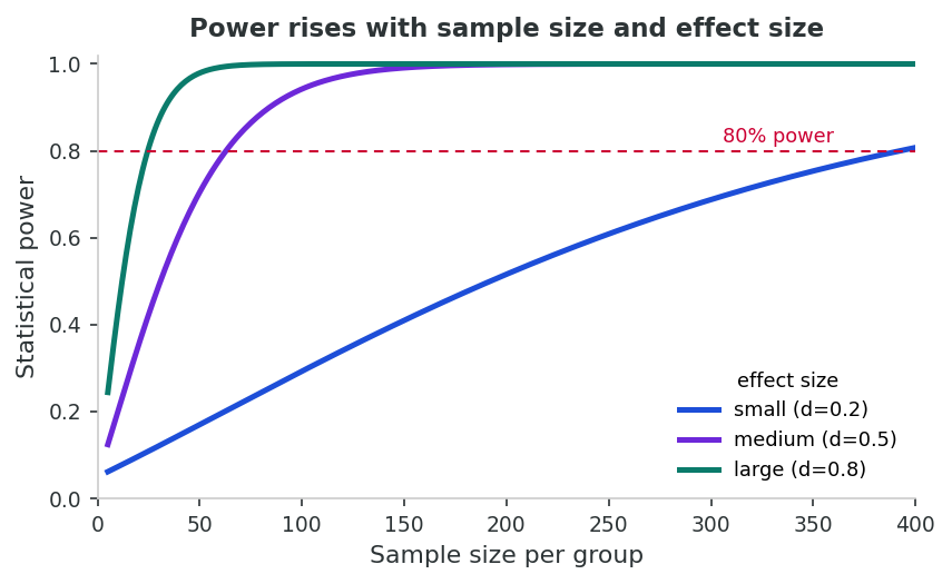
Rare disease studies are particularly vulnerable because small sample sizes mean low statistical power. A study of a disease affecting 1 in 100,000 people may have only 50 cases, yielding power of 20–30% for moderate effect sizes, meaning 70–80% of true treatment effects will go undetected. Paradoxically, the studies that do find significant results in low-power settings tend to overestimate effect sizes, a phenomenon called the “winner’s curse.” (Multiple testing, p-hacking, and the broader integrity issues these problems create are addressed in an earlier lesson.)
Simpson’s paradox occurs when a trend that appears in aggregated data reverses when the data are stratified by a confounding variable. The paradox highlights the danger of drawing causal conclusions from aggregate statistics without considering underlying group structure.
Consider a new treatment tested at two hospitals. Hospital A treats mostly mild cases; Hospital B treats mostly severe cases. Overall, Treatment X appears to have a lower success rate than the standard. But when stratified by severity:
| Group | Treatment X Success | Standard Success | Interpretation |
|---|---|---|---|
| Overall | 55/100 (55%) | 63/100 (63%) | Standard appears better |
| Mild cases | 27/30 (90%) | 51/60 (85%) | Treatment X is better |
| Severe cases | 28/70 (40%) | 12/40 (30%) | Treatment X is better, but is given to more severe cases |
The reversal occurs because Treatment X was disproportionately assigned to severe cases (which have worse outcomes regardless of treatment). The aggregated data hides this confounding by severity, producing a misleading conclusion. The correct causal interpretation requires stratification.
What you'll do: the simulator below builds a two-stratum population and lets you set how strongly the confounder drives both treatment assignment and outcome risk. What to take away: within-stratum risk ratios and the crude (unadjusted) risk ratio can disagree dramatically with each other and, with the right combination of strengths, can have opposite signs, the formal definition of Simpson's paradox. The simulator complements the R-box from an earlier section: there you stratified to recover a true null; here you can build sign-reversal by hand.
A two-strata population (e.g., mild vs. severe cases). Set how strongly the confounder C drives treatment assignment and how strongly C drives outcome. Watch the crude RR drift away from the stratum-specific RR. Push both sliders hard and you can flip the sign, Simpson’s paradox in action.
Green bars = within-stratum RRs. Red bar = naive crude RR ignoring the confounder.
Simpson's paradox is what happens when stratification reveals confounding at the individual level. The complementary problem is what happens when we move between levels of analysis, from groups to individuals or vice versa. Lesson 6 introduced this material in detail; the next two subsections recall the essentials.
The modifiable areal unit problem is a form of the ecological fallacy specific to spatial analysis. When individual-level data are aggregated into geographic units (census tracts, counties, provinces), the choice of unit size and boundary definitions can alter statistical results, sometimes dramatically.
A study examining cancer incidence near an industrial facility might find a significant cluster when data are aggregated at the postal code level but not at the health region level. Conversely, aggregating at a smaller level might produce unstable estimates due to small case counts. Neither result is “wrong”; both are artifacts of the chosen boundaries. The MAUP means that spatial epidemiological conclusions depend partly on arbitrary geographic decisions rather than solely on underlying disease patterns.
The ecological-fallacy and MAUP issues arise from how the data were assembled. The last analytic problem in this section is what to do when those data have holes in them, a near-universal problem whose handling can either preserve or wreck a study's conclusions.
Missing data are ubiquitous in epidemiological research. The validity of analysis depends critically on the mechanism underlying missingness; the modern taxonomy of MCAR / MAR / MNAR was set out by Rubin (1976):
Data are MCAR when the probability of being missing is unrelated to both observed and unobserved data. Example: a lab sample is accidentally dropped. Complete case analysis is unbiased under MCAR but loses power.
Data are MAR when missingness depends on observed variables but not on the missing values themselves, after conditioning on observed data. Example: younger participants are more likely to skip a depression questionnaire, but among people of the same age, missingness is unrelated to depression severity. Multiple imputation and maximum likelihood methods produce valid estimates under MAR.
Data are MNAR when missingness depends on the unobserved values themselves. Example: people with severe depression are less likely to complete follow-up questionnaires because of their depression. No standard analytic method can fully correct MNAR; sensitivity analyses with different assumptions about the missing data mechanism are essential.
When data are MAR or MNAR, restricting analysis to complete cases introduces selection bias. The remaining sample is no longer representative of the study population. For example, if sicker patients are more likely to drop out of a clinical trial, complete case analysis overestimates treatment effectiveness. Multiple imputation, which generates plausible values for missing data based on observed relationships, is preferred for MAR data.
Think of a health study you have encountered (in this course or elsewhere). Identify one potential statistical or analytic issue discussed in this section (model misspecification, multicollinearity, low power, Simpson’s paradox, ecological fallacy, MAUP, or missing data) that could threaten its conclusions. Explain why the issue applies and how it might have been addressed.
1. A researcher models the relationship between alcohol consumption and mortality using a linear regression and concludes that alcohol is uniformly protective. What error has likely occurred?
2. A treatment appears worse than the standard in overall data, but better when results are stratified by disease severity. This is an example of:
3. In a clinical trial for a rare disease with only 40 participants, which statement is most accurate regarding statistical error?
This lesson completed the bias inventory of this course by closing out confounding (an earlier section) and the analytic issues that survive even unbiased data (an earlier section). The HRT / WHI story made vivid how confounding can reverse the direction of a clinical recommendation, while confounding by indication and time-varying confounding showed why specialised tools, including restriction, active comparators, and marginal structural models, are part of the modern epidemiologist's repertoire. The lesson also pushed past the conventional “variable-by-variable adjustment” framing to ask harder theoretical questions about whether race, gender, and SES belong in models as confounders to be controlled or as structural exposures to be measured.
An earlier section then walked through the analytic problems that remain even after confounding has been handled: model misspecification, multicollinearity, Type I/II error and the winner's curse, Simpson's paradox, the ecological and atomistic fallacies, the modifiable areal unit problem, and missing data. These issues are the most common reasons a result fails to replicate, and recognising them is the last skill the course owes you before the integrated appraisal of a later lesson. The reflection below asks you to apply the full bias inventory to a study of your choice; the final assessment then tests the conceptual material before a later lesson integrates the entire course into a single critical-appraisal exercise.
The companion R script r-activities/HSCI_230_Lesson_11_Confounding_and_Statistical_Inference.R simulates a 5,000-person cohort in which SES drives both HRT use and CVD risk, but HRT itself does nothing. You will see the crude OR look strongly “protective,” the stratum-specific ORs sit near 1.0 (the truth), and the SES-adjusted OR recover the null, a hands-on reproduction of the HRT/WHI reversal that anchored an earlier section.
set.seed(230)
n   <- 5000
ses <- rbinom(n, 1, 0.5)                                   # 1 = high SES
hrt <- rbinom(n, 1, prob = ifelse(ses == 1, 0.6, 0.2))     # high SES uses HRT more

# CVD risk: lower in high SES, NOT affected by HRT (true null)
cvd <- rbinom(n, 1, prob = ifelse(ses == 1, 0.05, 0.15))

# Crude (unadjusted) OR -- looks "protective"
exp(coef(glm(cvd ~ hrt, family = binomial))["hrt"])

# Within each SES stratum -- the true effect: ~1.0
tapply(seq_len(n), ses, function(i) {
  exp(coef(glm(cvd[i] ~ hrt[i], family = binomial))[2])
})

# Adjusted OR, controlling for SES
exp(coef(glm(cvd ~ hrt + ses, family = binomial))["hrt"])Of the confounding-type and statistical-inference threats covered in this lesson, which do you believe poses the greatest practical risk to a typical observational study you might encounter in the public-health literature? Explain your reasoning, drawing on at least two specific examples from the lesson.
1. A variable is a confounder if it is associated with the exposure, is an independent risk factor for the outcome, and:
2. The WHI trial showed that HRT increased cardiovascular risk, whereas prior observational studies suggested a benefit. The key difference was:
3. Confounding by indication is best described as:
4. Marginal structural models address time-varying confounding by:
5. A study models alcohol consumption as a linear predictor of mortality and concludes alcohol is uniformly protective. The most likely issue is:
6. In environmental health research, including PM2.5, ozone, NO2, and SO2 simultaneously in a regression model may produce unstable coefficients because of:
7. States with higher income inequality have higher mortality rates. Concluding that individual inequality exposure harms individual health illustrates:
8. Concluding that raising every individual’s income will proportionally improve population health, based on individual-level data showing income predicts health, illustrates:
9. A cancer cluster study finds significant clustering at the postal code level but not at the health region level. This reflects:
10. Sicker patients drop out of a clinical trial more frequently. Analyzing only those who complete the study most likely produces: